Basic Elements of Machinery Diagnostics: An Overview 

In the machinery condition monitoring blog (a part of the Rotating Machinery Diagnostics Series), the focus of the discussion was on defining, characterizing, and implementing systems for monitoring rotating machinery during operation.

Such a programmatic approach provides, among other things, a way of organizing and directing technical resources so as to ensure maximal mechanical reliability and up-time for the monitored machines. It was stated that of all monitored parameters, vibration was the single most useful in diagnosing the broadest range of mechanical faults. That being said, what does it mean to diagnose faults in machines, and how is doing so facilitated by analyzing machinery vibration data?  This blog will cover:

1. Machinery diagnostics can be defined as follows
2. Machine Frequencies 
3. Vibratory Forces & Motion 
4. Selection of Vibration Measures & Frequency Spans 
5. Machinery Fault Diagnosis
6. Conclusion

Machinery diagnostics can be defined as follows: 

The utilization of machinery performance data in combination with technical knowledge and informed judgement to draw meaningful conclusions about the overall health of the machine, as well as the determination of mechanical faults, their causes, and their solutions.  

 From here onward, the term “machinery diagnostics” will be used synonymously with “rotating machinery diagnostics”. This is because the majority of the methods and technologies used and developed for machinery diagnostics are based upon and applied to rotating machinery. This in turn, reflects the primacy of rotating machinery and its central role in enabling the continuity of modern, organized human life. Rotating machinery plays an integral and vital role in everything from electric power generation to the manufacturing of semiconductors. It is because of this that machinery diagnostics has an essential economic component, as well as a critical safety component.  

 Machinery diagnostics is described by several authors as being inherently reactive in nature. While this isn’t entirely wrong, it is oversimplified. For the purposes of this discussion, machinery diagnostics will be divided into three distinct (but overlapping) areas of application:  

• Reactive Diagnostics  
• Proactive Diagnostics 
• Predictive Diagnostics  

Reactive Diagnostics

Reactive diagnostics can be thought of as “passive defense” and/or performing damage control. In such a situation, a machine will likely have broken a set vibration threshold, may be making excess noise, or the process that the machine facilitates may have become significantly degraded. In response, additional vibration data will often be taken in conjunction with some form of remedial action (ex. adjusting machine speed). Such an approach also extends to post-failure scenarios, where machine performance data would be analyzed in the time frame leading up to the failure to determine the root cause. While far from ideal, many (if not most) end-users tend to take this approach to machine diagnostics, often with higher monetary costs and at greater risk to the machine.  

Proactive Diagnostics 

 Proactive diagnostics can be thought of as “active defense” and seeks to both identify and interdict mechanical faults in the earliest stages possible. In such a situation, a machine may be functioning in a satisfactory manner, but upward trends in overall vibration corresponding to a monitored frequency may have been observed, and there may also be changes in other monitored parameters. In response, vibration and other performance data is analyzed in real-time to identify and resolve the root causes before they become a threat to the machine.  

Predictive Diagnostics

 Predictive diagnostics or prognostics extends the “active defense” posture that characterizes proactive diagnostics and can be thought of as “offense”. The logical extension of a proactive approach to fault detection is to accurately predict when and where faults might occur, and ideally the type and severity of the fault. Making such predictions requires analyzing and correlating large amounts machinery performance data, and predictive diagnostics leans heavily on machine learning & pattern recognition to achieve this aim.  

 Much of the remaining discussion about diagnostic methods will be based upon the reactive and proactive approaches, as both methodologies are the most common, the most accessible, and as of the time of writing the most widely used.  

Machine Frequencies  

Before proceeding to a detailed discussion of fault diagnosis, it is necessary to define the mechanical frequencies that will be used to identify machine faults. Every machine will have a very large (technically infinite) number of natural frequencies, as well as specific operating frequencies identified with the range of operating speeds, though only a few (typically the lowest) of the former are of interest. For diagnostics, the reference frequency is the machine operating speed (1X), and faults will often be discussed in terms of machine speed and integer or fractional multiples of it. It is common for condition monitoring systems to display speeds in terms of revolutions per minute (RPM) or the equivalent cycles per minute (CPM), and for frequency data to be displayed in terms of Hz (s^-1). Both are related by N_RPM = 60f_Hz.  

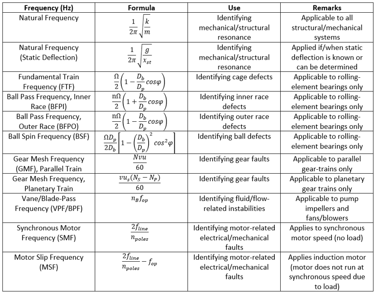Table 1: Commonly used frequencies for vibration-based diagnostics 

The parameters used in the formulas in Table 1 are defined and summarized in Table 2 below:  

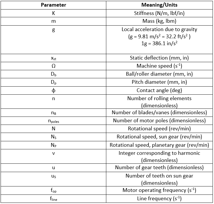Table 2: physical parameters for vibration frequencies 

 It should be stated that neither Table 1 nor Table 2 are exhaustive in nature. That is to say that there can be (and often are) other frequencies of diagnostic importance. Also, the above tabulated formulas and parameters do not explicitly take account of fluid-added mass effects on machine frequencies. Such effects are important in fluid-handling machinery where the fluid is incompressible (ex. boiler feedwater pump). The effects of fluid-added mass/stiffness/damping on vibration response will the subject of a future blog.    

Vibratory Forces & Motion 

The vibration response of any piece of rotating equipment is dominated by three major parameters and their corresponding forces: mass, stiffness, and damping: 

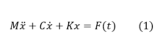
 A modified form of Equation 1 that does not explicitly rely upon the damping coefficient C is given by the following: 

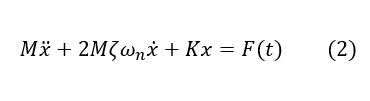
  The form used in Equation 2 is often more convenient because the damping factor ζ, which is itself dimensionless, can be determined directly via testing and/or measurement. In theory, the forcing function can take any mathematical form, but in applications involving rotating machinery vibration it will typically be of the form F(t) = F₀cos(ωt), where F₀ is the force amplitude and ω is the forcing frequency. The relation between mass, stiffness, and damping forces are shown in the figure below and are summarized in Table 3.  

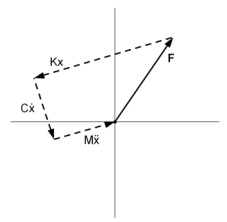
Figure 1: Vibratory force vector diagram 

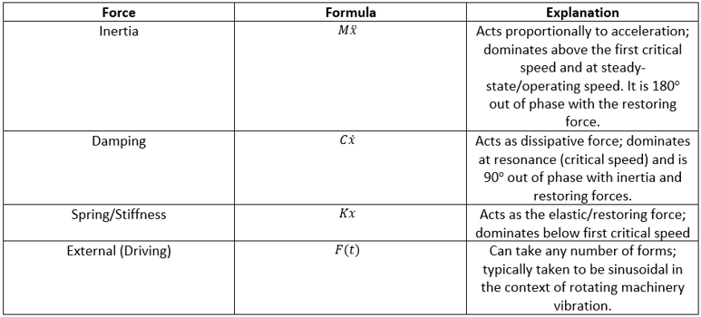Table 3: Vibratory forces 

Note that we take the rotor stiffness and damping to be linear (that is, proportional) to displacement and velocity respectively. While these assumptions suffice for many important practical applications of machinery diagnostics, there are situations of practical interest where the system behavior is non-linear, and the assumptions of linear stiffness and damping can lead to incorrect diagnoses. One common example is fluid-induced instabilities (oil whip and oil whirl) in fluid-film bearings. In this case, the nonlinearity will manifest as a spike at approximately 0.47X, or about 47% of the machine operating speed. Counter-intuitively, non-linear stiffness effects can arise in anisotropic linear systems. This is an academic way of saying that the stator/support stiffness, while linear, both differ in value with respect to a directional dependency. This anisotropy can be destabilizing and shows itself most transparently as a rotated/deformed ellipse in an orbit plot. Vibration data forms and presentation will be discussed in later sections. For now, it is fair and accurate to say that rotating machinery vibration is inherently non-linear, that rotors are inherently unstable systems, and that linearity is reasonable assumption in many practical cases that will yield accurate results for machinery diagnostics purposes.  

 Vibratory motion, or kinematics are of high importance, because vibration probes measure displacement, velocity, and acceleration, and vibration levels/thresholds are established and discussed in the same terms. The relations between displacement, velocity, and acceleration are summarized in Table 4 below.  

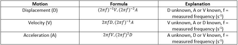Table 4: kinematic relations between displacement, velocity, and acceleration 

Table 4 is specific peak values of displacement, velocity, and acceleration. The Synchronous Vibration Cheat Sheet accompanying the Synchronous Vibration blog provides a comprehensive summary of kinematic relationships pertaining to sinusoidal vibration. Note that we can go between peak and root-mean-square (RMS) values by multiplying/dividing by 1.414 ≈ 2^1/2 and that peak-peak (pk-pk) values can be obtained by multiplying the peak value by a factor of two.   

Selection of Vibration Measures & Frequency Spans 

The accuracy of any analysis of a machine based on vibration data ultimately depends on the quality of said data. Since the quality of the vibration data depends upon how it is acquired and processed, it can be concluded that the accuracy and added value of any vibration analysis comes down to how the data has been acquired and processed.  

 Vibration data is acquired from a machine by a transducer that converts the vibratory motion into an electrical signal. The data acquisition system consists of the transducer, connections (hard-wire or wireless), processor, and the display/user interface. The most important factors to consider are the selection and mounting of the transducer. To properly select a transducer, one first has to decide upon what is to be measured (displacement, velocity, or acceleration), because each requires a different transducer, and each transducer achieves its optimal response in a different frequency range. The relationships among measures, applicable frequency spans, transducer types, applications and physical parameters are summarized in Table 5 below. These relationships provide general guidelines to transducer selection based upon the aforementioned factors. Improper selection and mounting of a transducer will almost always result in unreliable data.  

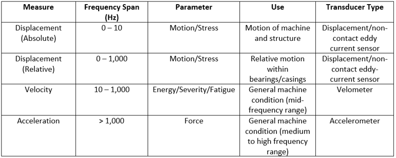 Table 5: Vibration Measures 

 For vibration measurements in rotating machinery, it is standard practice to use displacement sensors for vibration measurements taken directly from the shaft (ISO 7919), and to use velometers or accelerometers for measurements taken from the bearing or casing (ISO 10816).  

 This leads us to ask how best to determine frequency spans that will correspond to the selected measure and transducer. Doing so requires consideration of the dynamic range, data acquisition time and the spectral resolution. Default frequency spans that are broadly applicable for machinery vibration measurements are summarized in Table 6 below. These values are not ironclad and may have to be adjusted on a situational basis.   

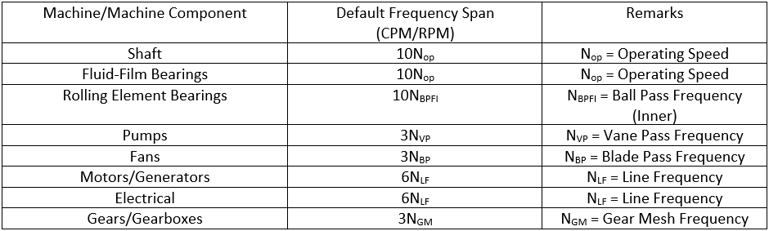Table 6: Default frequency spans for data collection (CPM/RPM) 

 The corresponding values in Hz (s-1) are obtained by dividing each CPM value by 60.  

 The relations summarized in Table 5 and Table 6 represent baseline requirements for the capture and processing of machinery vibration data. Excellent explanations of signal processing for vibration data analysis can be found in several other enDAQ blogs, including Spectral-Domain Time-Series Analysis by Strether Smith.  

Machinery Fault Diagnosis 

The ultimate purpose of machinery diagnostics is to make accurate statements about the condition of the machine based upon machine data. We want to know if vibration is excessive (i.e., in violation of established alert or alarm setpoints), and if so, at which frequency. It is also beneficial to have a many different ways of visualizing the data as is practical. Note that we said practical and not possible. It is all too easy to set up a situation where the capture and analysis of machinery vibration data becomes analogous to drinking from a firehose, with large (and expensive) data acquisition systems drawing huge amounts of data and generating esoteric plots that are often of questionable utility for the individual conducting the analysis. When it comes machinery vibration analysis, the quality of the data is of greater added value than the quantity or amount of data.  

 Four major forms of vibration data and analyses are tabulated below. Examples of these forms will be provided later in the section, with emphasis placed on the FFT/spectrum, as this is the most common plot used in frequency analysis, and frequency is the single most important parameter to consider when diagnosing machine faults.  

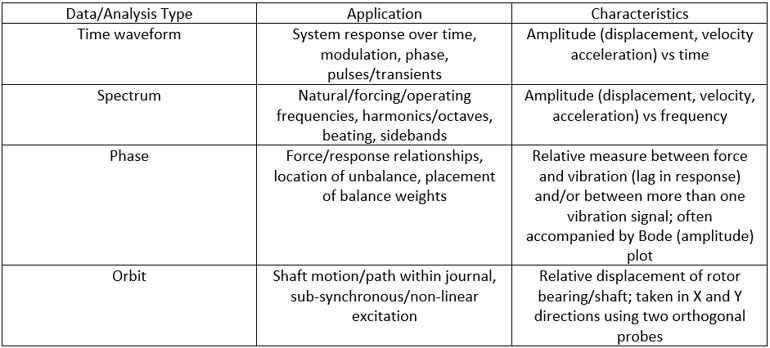Table 7: Data forms/diagnostic techniques 

 The data and analysis forms summarized in Table 7 are among the most commonly used in machinery diagnostics, with frequency spectra being the most common and the time waveform running a close second. Orbit analysis requires that two mutually orthogonal probes be set up in a fixed position (ex. within the bearing housing or pedestal) and situated orthogonally to one another. Non-contact eddy-current sensors calibrated in accordance with an appropriate gap voltage (ex. mV/mil) are the most common types of probes used for this purpose. This type of probe/configuration is most often seen at land-based power generation plants featuring large (300 MW) gas/steam turbine generator sets. Examples of the various data types are shown in the figures below.  

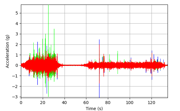
     Figure 1: Acceleration time waveform (enDAQ) 

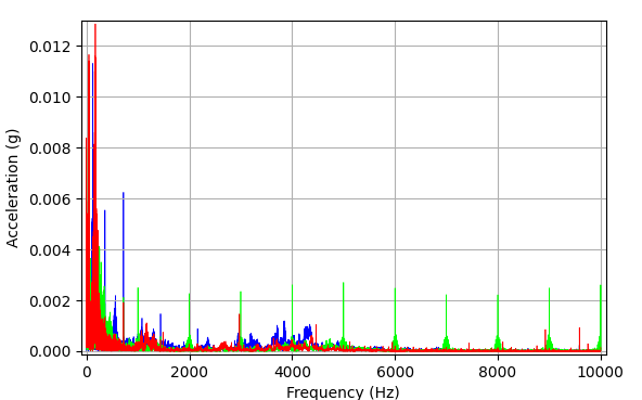
         Figure 2: Acceleration spectrum (enDAQ)

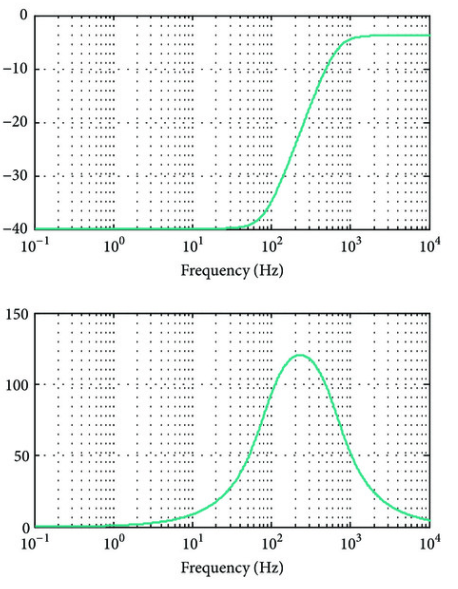
Figure 3: Sample Bode plot, phase top, amplitude bottom 

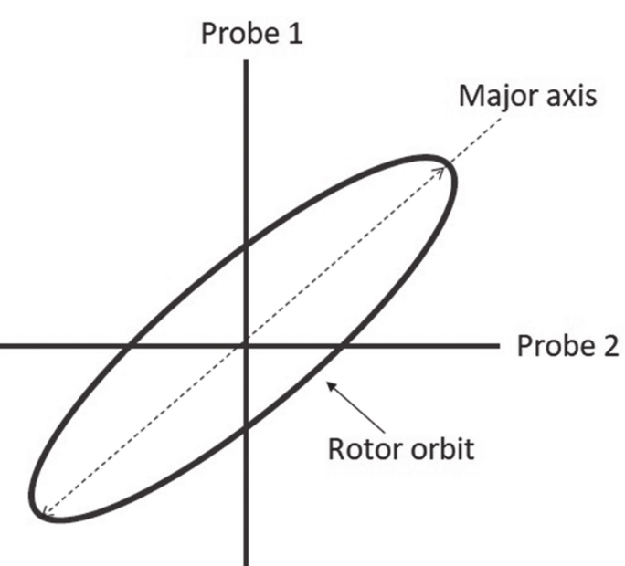
  Figure 4: Idealized rotor orbit plot, filtered to 1X

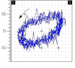
Figure 5: Representative “real world” orbit plot

It is readily seen from Figures 1-4 above that vibration data can take many forms, and in real-world applications both in the lab/shop and in the field at the point of application, said data can be quite messy, and may not indicate at first glance what potential problems the machine may have. Different plots also add value to the diagnosis in different ways. For example, in the phase/bode above, what diagnostician is looking for is the relation between the amplitude spike or “bump” in relation to the phase change, with is often indicates a resonance condition, the most obvious example of which is during start-up when the machine passes through the first critical speed. The orbit can be used assess the amount of anisotropy and is a powerful tool in diagnosing shaft cracks. The value of the time waveform and spectra is in their commonality, usability, and the relative ease with they can be processed and analyzed. This is especially true of the frequency spectrum, which be main focus of the rest of this section and the basis for diagnostics & troubleshooting tables that follow.  

 The analysis of frequency spectra will almost always include some or all of the following steps: 

• Determine machine operating speeds and multiples (orders) of the operating speeds. 

• Determine dominant frequencies that are multiples of the operating speed and are specific to the machine (ex. vane-pass in pumps, gear mesh in gears, etc.) 
• Determine non-synchronous/sub-synchronous multiples of operating speed (important in the diagnosis of fluid-related instabilities).  
• Determine beat frequencies (“beats” are two frequency components in close proximity to one another, sometimes referred to as “quasi-resonance”).  
• Determine any frequencies not directly dependent upon machine operating speeds, such as natural frequencies, frequencies of nearby machines, electrical frequencies, piping frequencies, etc.  
• Determine sidebands that correspond to low-frequency vibration components and/or other frequency components specific to the machine type (ex. gear fault may show up with spikes at the gear-mesh frequency with sidebands at 1X). 

 The series of tables below summarize mechanical faults as they relate to specific machine frequencies and provide basic troubleshooting guidance.  

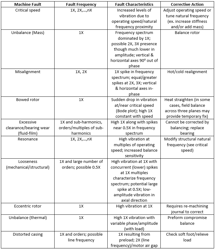Table 8: Operating speed faults 

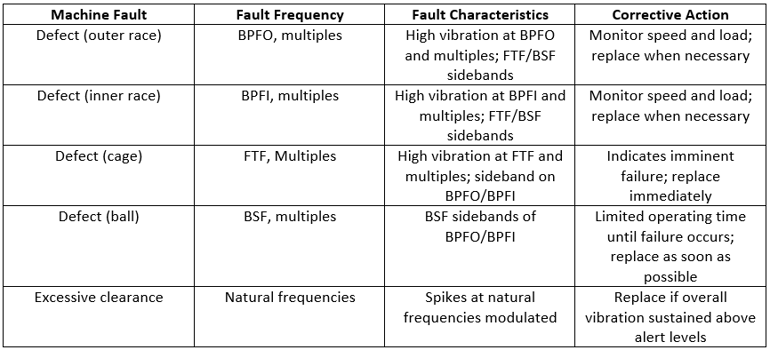 Table 9: Rolling element bearing faults 

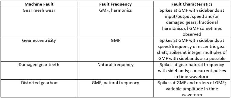 Table 10: Gearbox faults 

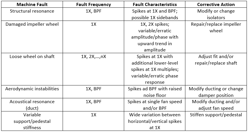 Table 11: Fan faults 

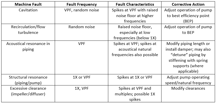 Table 12: Pump and piping faults 

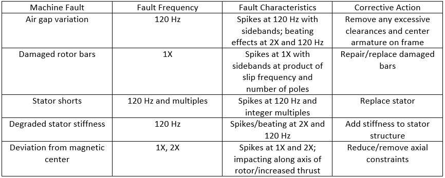Table 13: motor faults 

Conclusion 

It is hoped that the information provided here will be of practical use to those tasked with diagnosing and troubleshooting problems with rotating machinery laboratory, plant, shop, and other industrial environments. It is also hoped that the information contained herein has provided useful introduction for those new to machinery diagnostics.  

Rotating Machinery Diagnostics Series

This post is part of the Rotating Machinery Vibration Series. Feel free to check out my other related posts;

• Overview of Synchronous Vibration - Plus Cheat Sheet
• Gear Noise & Vibration: Why it is Important
• Machinery Condition Monitoring: A High-Level Overview
• Undamped Critical Speeds for Simple Rotors