The Vertical Direction: Measuring the Amplitude of the Signal

In previous blogs, I have discussed a variety of issues that must be addressed to acquire good-quality experimental data. However, I have never covered the real objective: Characterizing the amplitude of the phenomenon of interest.

 This discussion will cover:

1. The Objective of Data Acquisition
2. Errors
3. Signal-to-Noise Ratio and Range-to-Noise Ratio
4. Our Experiment
5. Analog Errors
6. Quantization Errors
7. Errors that Occur During/Because of Excitation
8. How Well Does a Real Data System Do?
9. The Effect of Bandwidth on Noise
10. What should our Measurement Strategy Be?
11. Let's Model an Experiment.
12. Out-of-Band Energy
13. A System Design Philosophy
14. Headroom
15. A Second Horror Story
16. Conclusion 
17. References

The Objective of data acquisition

The basic objective of data acquisition is to quantify the amplitude of some phenomenon. For many applications, we use a digital data acquisition system to do it. The system takes a series of "snapshots" of a signal, called samples, that are repeated to produce a time history. The result is analyzed to characterize the phenomenon of interest.

The rules that govern the requirements for how fast samples must be taken are the subject of a myriad of papers including some of my earlier blogs. For this discussion, we will assume that the requirements have been satisfied. Here we will discuss the critical aspects of the amplitude-quantification process.

We will cover three fundamental issues:

• The measurement objective: Obtaining consistently useful data.
• Problems, if not handled properly, will make our data questionable or unacceptable.
• Good practices: What do we need to do to improve our chances of getting good data?

This is obviously an enormously complex problem if we don’t limit ourselves to a relatively small set of applications. For the purposes of this discussion, we will concentrate on mechanical tests in the audio frequency range: 0-100KHz, such as acoustics and mechanical vibration and shock. We will use examples from that regimen.

What we want is a measurement that does not have the significant errors shown in Figure 1.

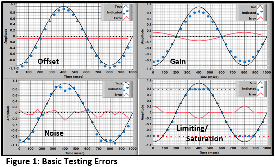
The measurement should:

1. have correct gain and offset (calibrations and/or corrections).
2. be significantly greater than the noise level (giving a satisfactory signal-to-noise ratio (SNR).
3. be within the measurement system's range.

Failure to meet any of these objectives will produce poor results.

The first requirement should be satisfied by proper calibration, a subject for another day. This paper concentrates on the second and third items. Our objective is to get a satisfactory SNR without limiting/clipping.

Here we will discuss three parameters that must be handled properly to assure a good data set:

1. Measurement full scale (the maximum signal you can measure).
2. Measurement maximum signal (the maximum signal you expect).
3. Noise, which introduces uncertainty into our measurement, and its two main sources:
1. Analog: Electrical noise from a variety of sources.
2. Digital/Quantization: Noise that comes from the quantization process.
4. Errors induced by/during the experiment actuation.

Signal-to-Noise Ratio (SNR)

                 and Range-to-Noise Ratio (RNR)

The end objective of our experiment is to get a satisfactory Signal-to-Noise Ratio: SNR. However, the parameter that we will define and discuss here is the Range-to-Noise Ratio: RNR, which is a characteristic of the instrumentation and data acquisition system.

The basic definition of RNR is:

RNR=RMS(Measurement Range)/RMS(Noise)

By convention, we assume a sinusoidal full-scale signal and define:

RNR=RMS(Sin(Full Scale))/RMS(noise)
=.707 x Full Scale/RMS(Noise).

A good RNR is required to produce a satisfactory SNR.

Anyone reading this article probably uses a measurement system that looks like Figure 2.

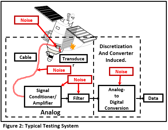
All of the components contribute to errors in our measurement. They are of two types: Analog and Digital.

Analog errors (noise) are introduced in the transducer, cabling, and signal conditioning/analog-filtering operations. The errors will depend on the combination of devices in the signal train. The noise comes from a variety of sources (Reference 1):

• When a current is passed through a resistor the voltage will be the expected “E=IR” plus some noise. The cause of the noise is under debate, but its characteristic is well defined: at low frequency, its spectral magnitude rolls off proportionally with frequency. It is called 1/f or Pink Noise.
  If a resistor alone produces noise of this sort, a circuit of multiple components will produce more.
• The background environment will produce noise whose spectral magnitude is approximately constant with frequency. This is called Thermal or Broadband Noise.

The combination of 1/f and broadband noise produces a signal with a spectrum that looks like Figure 3. (Note that it’s not really 1/f.. its k/f where k is a characteristic of the device/system.)

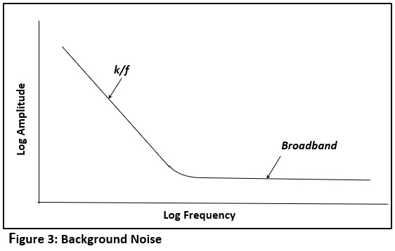
Figure 4 shows the spectral noise (PSD) characteristics of a structural-dynamic-test setup measured with the accelerometer at rest.

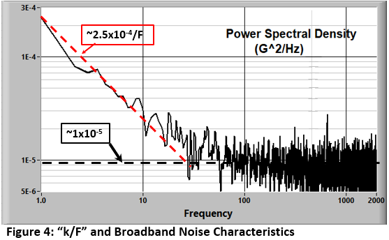
The noise includes contributions from the transducer, cabling, and signal conditioning. In this case, k/f noise dominates out to about 20 Hz where the characteristic changes to “broadband”.

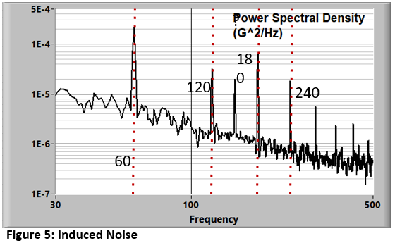
• Local influences that produce electrical and magnetic fields will produce errors called Induced Noise. If we are using a system that has a wired connection between the transducer and data system (as most of us are) electrical and magnetic fields near the cabling will induce noise. Figure 5 shows 60Hz (and harmonics) noise that should be reduced if it is significant relative to full scale.
  
  

Overall result: My experience is that in a well-designed and executed general laboratory experiment, the analog noise level within a 20KHz. bandwidth is of the order of 0.001V RMS.

The concept of analog-to-digital conversion is straightforward: A hardware device (Reference 2) converts a real (continuous) signal into a series of discrete (time and amplitude) values.

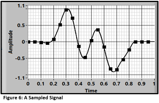
The first step is to sample the data. Figure 6 shows the result of sampling a waveform at 10 samples/second.

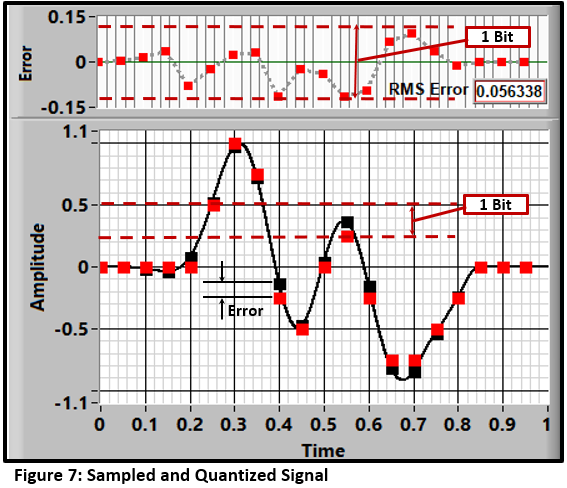
The next step is to quantize the samples. For most systems, the result is a set of binary numbers: 2^N (where N is the number of bits) discrete values spread between the negative and positive voltage limits of the measurement. The result for a 3-bit (8-step) quantification is shown in Figure 7. The difference between the sampled version (black squares) and the quantized set (red squares) is the quantization error (upper frame). 

Step Size=Range/2^(N) ~Error (RMS)

Table 1 shows the discretization step size for systems with different bits and full-scale voltage combinations. The RMS error is approximately equal to the step size (Reference 5).

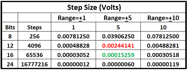
The result is that for 5 volts full scale (matching the full-scale of many transducers):

• the 12-bit system is “noisier” than the typical 1 mv analog noise.
• 16-bit resolution produces discretization noise that is normally much less that the analog contribution.
• a 24-bit system introduces insignificant noise.

The simplest method of assessing the total noise in a measurement system is to apply a quiescent input and look at the result. For the system in Figure 2, we would put the accelerometer on a pillow and acquire a data set.

Assessing the system's accuracy for a dynamic signal requires a more complex test. One possibility, that evaluates the capabilities of the data acquisition system alone, is the "Effective Bits Test" (Reference 6). We will discuss this technique in a later blog.

There are a variety of additional errors that may occur when the test is executed:

• Non-Linearity: We assume that all of the measurement components have an indication that is directly proportional to the actual physical input. Deviations will cause distortions in the time history and spectral measurements. If known, they can be corrected in post-processing.
• Transducer Resonance: All mechanical transducers have resonant frequencies. If not measured or adequately suppressed, they will cause errors within the bandwidth of interest. In some cases, these errors can be mitigated by post processing (Reference 10).
• False signals generated by transducer base strain. 
• Cross-axis errors (response to motions perpendicular to the nominal axis). These can be compensated if known.
• Triboelectric effects generated by cable motion.
• Electromagnetic fields produced by explosive actuation. Plasma in the area of the transducer will cause broadband noise. Proper shielding of the transducers and cabling will reduce the effects.
• Static electricity may be created by the deformation of polymeric foam padding and relative sliding of components against foam padding. This can cause both high and low-frequency distortions in data.

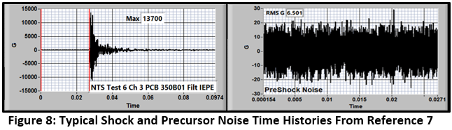
Let’s explore some real applications. Over the years I have collected pyroshock time histories that are representative of these nasty environments. They contain both the event time history and the quiescent noise in the event precursor. The data sets include the following transducers and data acquisition systems.

• 6 records from different transducers in the pyrotechnic shock test described in Reference 7: Signals from PCB 350B01, Endevco 7255A, PCB 350D02., Endevco 7270A, PCB 3991, and Endevco 7280A accelerometers were acquired with a Piranha sigma-delta-based data system.
  A typical result is shown in Figure 8.
• 1 record contributed by a reader using a PCB 3503A acquired with a DEWESoft oversampling data acquisition system.

A compilation of the results is in Table 2.

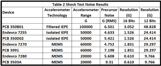
The critical point is that in every case, the measured RMS noise is significantly larger than the vertical resolution (Discretization RMS Error) for a 16-bit data acquisition system where each channel has a gain that covers the full scale of the transducer. 

The analog noise controls the range-to-noise ratio RNR (and SNR) in every case.

• More than 16 bits will not help the overall test accuracy significantly.
• At 12-bit resolution, the digitizing errors will control the accuracy.

So far, we have addressed the amplitude (vertical) characteristics of the measurement. However, to assess the success of our measurement, we also need to discuss the frequency (horizontal) characteristics of the signal and how the indicated noise is affected.

The frequency range of the measurement, called bandwidth, is a primary controller of the noise & resulting error in the experiment.

The noise of the experiment is the total of the noise/error spectrum over the measurement bandwidth.

This bandwidth of the measurement is defined first by the Nyquist frequency:

F_N=Sample Rate/2.

Our digital measurement system cannot see anything above that frequency. The alias-protection system (low-pass filter) will reduce it further (Reference 8).

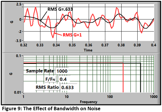
Performing a low-pass filter on the data will reduce the noise in the signal. Figure 9 shows the effect of filtering a 1G RMS signal that has a flat spectrum with a square low-pass filter at 40% of the Nyquist frequency.

The resulting RMS noise is: Input x √(F/FN)

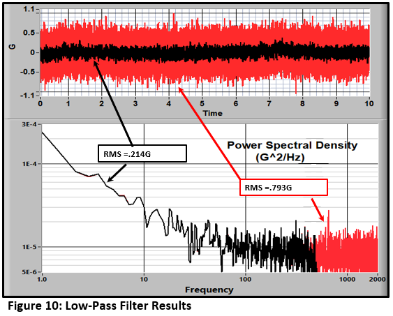
This idealized case never happens in the real world. Figure 10 shows the effect of a 500 Hz, 8-pole, Butterworth low-pass filter on a quiescent-excitation noise spectrum. The RMS noise is reduced from 0.793 to 0.241 Gs.

Let's lay out our objectives in more detail:

• Measure our time history with a satisfactory Signal-to-Noise ratio (SNR) for the bandwidth of interest. In previous blogs, we have called that F_D (Frequency Desired).
• Be sure that our data system amplitude limit is not exceeded (saturated) under any conditions.
• Ensure that our data set includes any surprises.
  • That is the point of testing… right?

Our test requester has said that the maximum frequency of interest is some value (F_D). We need to set our sample rate to more than twice that. Then, we need a low pass filter to assure that the data is not significantly aliased. The cutoff of the filter should be above F_D and the sample rate should be set at a value that depends on the anti-alias filter characteristics (Reference 9).

Strategy 1 -The Conventional Approach:

Let's look at a shock data set using the "normal" approach. Our requester has specified a 10KHz F_D. The expected response is less than 10,000 Gs. We use a 50KG accelerometer and set our amplifier gain to a range of +10,000G. We will use a good anti-alias filter set at 15KHz. that allows a sample rate of 40KS/S. Figure 11 shows the results. The measured response is well within the +10KG range, the spectrum is rolled off well below the Nyquist frequency, and the signal shape looks credible....

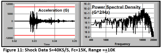
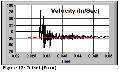
....but it's not right! 

If we integrate the measured acceleration into velocity, we get the curve in Figure 12. It indicates that the specimen is headed out of the laboratory at about 18 inches/second. This is probably not the case. That is an error. What's wrong? 

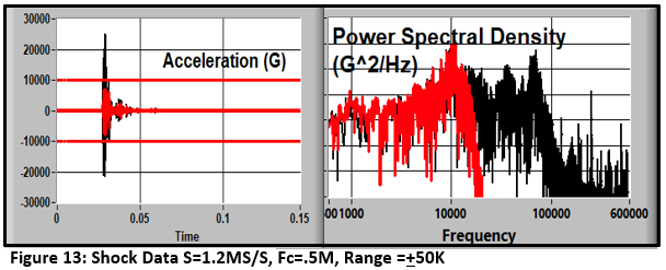
Strategy 2 - A Wider View:

If we acquire the data with a higher range (50 KG (matching the transducer capability)) and a higher sample rate (1.2 MS/S) we get a very different picture (Black curves in Figure 13). There is a transducer resonance near 70 KHz that produces a total response of about 25KG. With the gain used in the original "experiment", the input amplifier is saturated. But, because the low-pass filter smoothed the time history, we can't see it.

The resulting velocity (black curve) looks reasonable (Figure 14). 

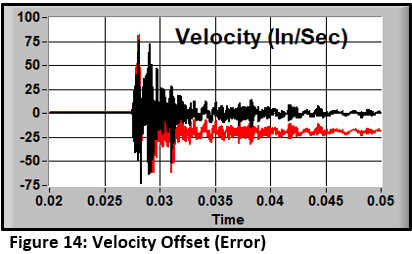
Acquiring at the lower rate and range resulted in a hard-to-detect, corrupted measurement.  

This data set may be digitally low-pass-filtered and downsampled to get the desired (correct) result. At the same time, any corrections for system transfer function distortions can also be done (Reference 10).

Restricting the measurement bandwidth to agree with F_D caused in-band errors and prevents the detection of high-frequency responses that may be critical to the test validity or actually be of later interest to your requester.

The villain here is called

Out-of-band energy is made up of signals that have a significant amplitude and a frequency that is higher than you expect or probably, care about, for your end result. The example above is a shock test where transducer resonance is the problem. But there are lots of other possibilities:

• In a temperature measurement where a thermocouple is used, the signal will often include power-line noise and its harmonics.
• Significant radio-frequency signals may be introduced by the fact that the signal lines are actually pretty good antennas.
• Electrical noise induced by an explosive environment.
• High-speed camera electrical and mechanical noise.

The system must be capable of handling these extraneous signals.

In addition, high-frequency signals can cause errors in the electronics due to slew-rate limitations. This issue is discussed in Reference 11.

Ideally, the data system should have a range and bandwidth that covers all of the "reasonable" possibilities.

The fundamental concept is very simple:

• Minimize the number of analog components in the system.

• Measure the response to the maximum bandwidth of the system to capture measurement anomalies such as transducer resonance.

• Measure to the full range of the transducer (of course, assuring that the transducer has adequate range).

• Do as many of the calculations as possible in the digital domain.

• Use an oversampling/Sigma Delta data acquisition system. As discussed in Reference 12, good systems provide a “nearly perfect” digitization of the input time history:
  • Essentially constant gain and constant delay result in nearly zero distortion.
  • Essentially perfect alias protection.
  • Digital implementation makes the systems immune to age effects (drift/gain).

  Systems with sample rates of up to 250,000 samples/second (bandwidth up to ~110 KHz) are readily available. Premium systems offer higher rates.

• Do NO analog filtering (other than the required pre-converter filter in an oversampling system).
  • Analog filters distort the data, add to the inherent noise, and hide out-of-band energy.
• Use a signal conditioner that matches the transducer capabilities.
  • Assure that it has adequate bandwidth to cover all potential anomalies.
• Do bandwidth and sample rate reduction in digital post-processing using proper filtering/downsampling processes (Reference 10).

• Your data set is bigger. Not a problem with most modern systems.
• Your data is noisier. If the background spectrum is flat, the noise level will increase by the √(bandwidth/F_D): ~3.1 for 10x upsampling assuming a flat noise spectrum.
  Not a big increase. With a good 16-bit (or higher) system, the dynamic range will provide a satisfactory SNR for the bandwidth of interest.

This approach results in another test planning feature that is critical if you don’t know what to expect. If the response (including transducer resonances and other anomalies) is larger than expected, the system may be saturated and cause hard-to-detect errors. If our bandwidth and range cover these signals, we can assure that there is no saturation.

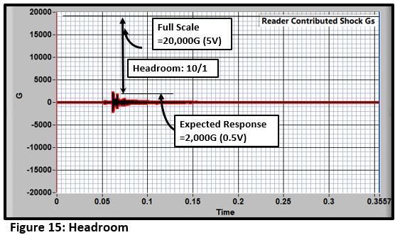
The ratio of expected response to full scale is called headroom. The bigger it is, the more tolerant the experiment is to surprises.

High-resolution data acquisition systems (16 or more, bits) allow us to use high headroom ratios. For example, if the expected response is 2000G, and the system range is 20KG, the headroom is 20000/2000 = 10 (Figure 15).

A Second Horror Story

In my last blog, I described a test series where poor headroom choices resulted in a very expensive error caused by aliasing. Here is another sad tale, caused by non-conservative scaling/inadequate headroom.

Several years ago, a laboratory was vibration testing a spacecraft on a horizontal slip table. To demonstrate the issue, we will assume that the objective was to drive the specimen to a few G’s. The test was set up with gains that produced a range of 5 Gs. This all sounds reasonable, but the slip table stuck and then released suddenly creating motions that saturated all of the channels in the drive direction. Consequently, they had no idea how hard the spacecraft had been hit. Was the specimen subjected to accelerations that were above its design limits? There was no way to tell. The result was a necessary (and expensive and program-delaying) tear-down of the spacecraft to find out whether there was damage.

If the test had been set up with a range that was greater than the design damage threshold, and the measurement showed that it had not been exceeded, the teardown/inspection might have been avoided. The data system’s dynamic range would have provided adequate resolution for the expected response if it was scaled to 50 Gs.

Scale for disaster. Accidents do happen. The capabilities of a good 16-bit system allow us to be very conservative in our scaling.

Conclusion

In this blog, I have discussed data acquisition strategies that I think are appropriate for structural dynamic testing. Other regimens obviously require different analysis, and perhaps, different approaches.

The critical point is that modern, high-quality data acquisition systems allow both conservative scaling and high bandwidth. If you use these systems properly, it will increase the probability that both the desired data and unexpected test phenomena are captured and characterized accurately. 

References

1. What Is Electrical Noise and Where Does It Come From?: All About Circuits, Robert Keim

2. Analog-to-Digital Converter: Wikipedia

3. Taking the Mystery out of the Infamous Formula, "SNR = 6.02N + 1.76dB," and Why You Should Care: Walt Kester, Analog Devices MT001

4. Quantization Noise: An Expanded Derivation of the Equation, SNR = 6.02 N + 1.76 dB: Ching Man, Analog Devices MT-229

5. A Different View of the Sampling & Quantization Process in Digital Data Acquisition: Strether Smith, EnDAQ Blog

6. Effective Bits, A Not-so-New Way to Characterize Data Acquisition System Accuracy: (PDF) Strether Smith 

7. Evaluation of Accelerometers for Pyroshock Performance in a Harsh Feld Environment: Anthony Agnello, Robert Sill, Patrick Walter, Strether Smith, PCB Piezotronics.

8. Sample Rate: How to Pick the Right One: Strether Smith, EnDAQ Blog

9. How Fast Must We Sample?: Strether Smith, EnDAQ Blog

10. Spectral-Domain Time-Series Analysis: Tools That Improve Our View and Understanding of the Data: Strether Smith, EnDAQ Blog
11. The Effect of Out-Of-Band Energy on the Measurement and Analysis of Pyroshock Data: (PDF) Strether Smith, 80th Shock and Vibration Symposium 

12. Sigma Delta Converters: Strether Smith, EnDAQ Blog