Sample Rate: How to Pick the Right One

In the last blog, we discussed the basics of sampling theory and demonstrated that, if there is any energy at frequencies above the Nyquist Frequency (F_N = Sample Rate/2), the data will be corrupted (aliased). There is always energy above F_N so there will always be errors. Now, we need to figure out what to do about it.

Acceptable Aliasing Errors?

Figure 1 shows the situation. The blue curve is the spectrum of the real data. If we sample at S samples/second, the spectral energy above the Nyquist frequency will fold around F_N and superimpose itself on the data below F_N as shown in the red curve. As we already know, there is aliasing error at all frequencies below F_N but, if the spectrum rolls off at high frequency (as shown), there will be a frequency range where the error is relatively small. We now need to define a level of Acceptable Alias Error. At what frequency is the aliasing small enough to accept? We will call this frequency F_A .. Our data is “Good” below that frequency and unacceptably corrupt above it.

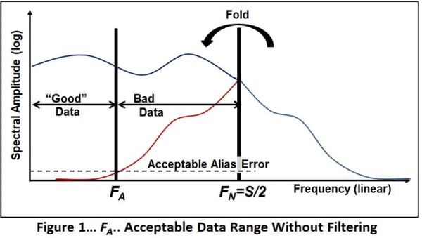
As we can see in this example, only a small part of the frequency range between zero and the Nyquist frequency is acceptable. What can we do to improve the situation?

Figure 2 shows the effect of applying a low-pass filter that has a cutoff frequency of F_C to the data.  The filter reduces the energy above the Nyquist frequency so that, when it folds, there will be less corruption below F_N. The frequency range with an acceptable level of aliasing is increased.

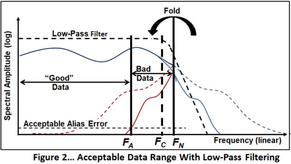
That’s the basic idea..

But we have asked the wrong question. We started with the sample rate and found out what part of the data range is “good”. It makes more sense to start with what we need and find the required sample rate.

Desired Bandwidth

The proper question is: What is the desired bandwidth? This is an engineering decision. Our objective is to acquire data that has aliasing error reduced to an acceptable level between zero frequency and the Desired Bandwidth (F_D).

But, it’s not that simple. The problem is that we don’t have a clue what the input spectrum is. So we will make the assumption that the signal has a spectrum that is flat over all frequencies. Most of the time this will be conservative because the spectrum normally rolls off above F_N (as it does in Figure 1) but this is not always the case. Let’s cross our fingers and press on.

Alias Mathematics

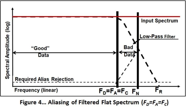
The “geometry” of the filtered flat spectrum aliasing is shown in Figure 3. From the symmetry of the aliasing, you can see that:

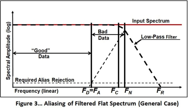
..where F_R is the frequency at which the filter has attenuated the input to the “Required Alias Rejection” level. (Note that we have changed from “Acceptable Alias Error” to “Required Alias Rejection” because now we are talking about rejection of aliasing error.. not the error itself.)

So, knowing our Desired Frequency Range (F_D) we can determine the Sample Rate (S) that is required for a given alias rejection from EQ 1.

That is pretty useful but there is another approach that is more informative. It is based on determining the minimum number of points/cycle at our Desired Bandwidth (F_D).

For this special case, we will set our Filter Cutoff Frequency to be the same as our Desired Frequency Range (F_D = F_C) as shown in Figure 4.  

Now, we define the Sample Ratio:

SR = Sample Rate/Desired Bandwidth = S/ F_D = Points/Cycle at F_D.

Next, the required Sample Ratio can be shown to be:

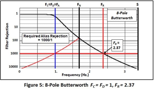
So, let’s look at the example of an 8-Pole Butterworth filter set at 1 Hz (Figure 5).

The black curve is the filter shape that, since we have assumed a constant input spectrum, is also the shape of the response spectrum. We will put F_c (-3dB) at 1 Hz. Next, if we use 1000/1 as our Required Alias Rejection we find that the filter meets this requirement at 2.37 Hz so F_R / F_D ~ 2.37. From Eq. 2, the required (minimum) Sample Ratio is ~3.37.

Most of the time, we will set F_D lower than F_C because we don’t want the filter to attenuate the data significantly in the frequency range we care about. So, this approach will normally give us a conservative Sample Ratio.

Bessel, Butterworth, Elliptical, Sigma Delta?

So, that’s what an 8-pole Butterworth filter does for us. We know that we have a myriad of other filter options. Figure 6 shows the attenuation characteristics for several high-end, commercially available, filters:

• 8-Pole Bessel
• 8-Pole Butterworth
• 8-Pole/8-Zero Elliptical (There are many flavors of the elliptical filter. This one is similar to the Precision Filters LP8).
• Sigma Delta (∑Δ) Emulation (There are also many versions of ∑Δ filters. This one is similar to the Analog Devices AD1974).

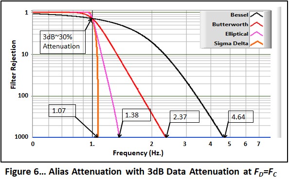
(Note: Different filter types have different definitions of the filter cutoff. These curves are adjusted so that the frequencies of the -3dB (Gain=.707) point agree.)

This is the case for F_C= F_D where the maximum filter attenuation is -3dB (~30%) within our frequency range of interest (30% error).

If we require less attenuation at F_D, we have to lower it to the point where the attenuation is acceptable. For instance, if we choose to allow only 10% attenuation at F_D, then the filter characteristics look like Figure 7. The required Sample Ratio is significantly higher for the Bessel and somewhat higher for the Butterworth options. The results for the sharper filters are essentially unchanged.

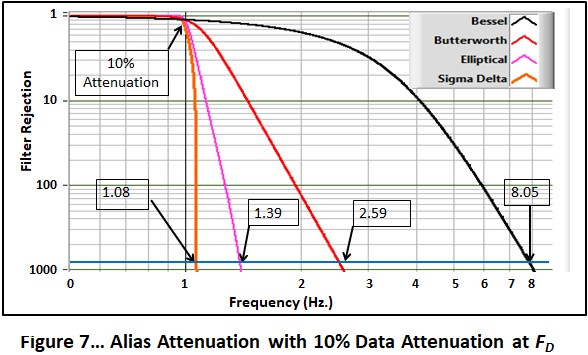
Now we will apply Eq 3 to calculate the required Sample Ratio for each of these results.

What we see is that, if we use a sharp filter (elliptical or Sigma Delta) we can acquire the data at significantly lower sample rates than for the “conventional” filters. In fact, the Sigma Delta filter gets very close to the ideal value of 2. With strong elliptical or ∑Δ filters, it is perfectly reasonable to use a Sample Ratio of 3 (I don’t recommend any less for reasons we will discuss in a later blog).

Summary

So, the process to determine the required sample rate is:

1. Decide what bandwidth you need (F_D). This is an engineering decision that will require some thought. In some cases, tradition may be the (dubious) decider. For instance, in spacecraft-component-vibration testing, an analysis bandwidth of 3 KHz is normally the goal.
2. Decide what Required Alias Rejection you need. I have used 1000/1 in these examples. Other possibilities are:
   1. The measured dynamic range (Full Scale/noise level) of your experiment. (This actually makes the most sense).
   2. The theoretical dynamic range of your data acquisition system.
      • 12 bits: ~ 1/4997
      • 16 bits: ~ 1/80030
        (Where did these come from: Tune into a later blog.)
   3. Find the required F_R from the Required Alias Rejection and the transfer function of the anti-alias filter.
   4. Calculate the Sample Ratio from Eq. 3. (If it is less than 3, round it up)
   5. Determine the minimum Sample Rate: S = SR x F_D
   6. Bump the number up a bit to be conservative. If your data acquisition system has discrete steps, use the next higher one.
      
      

OK, That's the Minimum Sample Rate

This process determines the minimum sample rate that you should use. Should you sample faster? It depends. A basic rule is that it never hurts to sample too fast. But, should you?

• If you are only going to do spectral calculations (Fourier spectra, PSD, SRS, N^th Octave..),
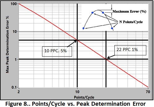
  3 points/cycle at F_D, are enough.
• If you are doing time domain investigations, you will normally need more points. An often-quoted rule is that you need 10 points/cycle at F_D to get a good representation. However, if you are interested in peak values, that is not enough. Figure 8 shows the situation when you are unlucky enough to have your data points equidistant on each side of the peak. At 10 points/cycle you will have a 5% error in peak determination. If you want to be assured that you capture the peaks to an accuracy of 1% you need a Sample Ratio of 22. 

If you are restricted in sample rate or data volume by your hardware, you may not be able to sample as fast you need to get the desired time-history amplitude resolution. In that case, upsampling (the subject of a future blog) will solve the problem. 

Conclusion (for now)

So, now I hope that you know that we need low-pass/anti-alias filters. Next, what kind should we use: Bessel, Butterworth, Elliptical, Sigma Delta, whatever. In our next blog, we will take a brief look at how analog and digital filters are “constructed” and then discuss my spin on which one(s?) you should, and shouldn’t, use. 

Send a Comment or Question to Strether

One of the reasons I've been writing these blogs is to get a discussion going. Please reach out privately to me with any questions or comments you may have.  

You can participate by:

• Entering comments/questions below in the Comments Section at the end of the blog. This will obviously be public to all readers.
• Contact me directly. I will respond privately and (hopefully) promptly. If appropriate, your question could be the subject of a future blog.

This blog is meant to be a seminar... not a lecture. I need your help & feedback to make it good!

Disclaimer

Strether has no official connection to Mide or enDAQ, a division of Mide, and does not endorse Mide’s, or any other vendor’s, product unless it is expressly discussed in his blog posts.

Additional Resources

If you'd like to learn a little more about various aspects of shock and vibration testing and analysis, download our free Shock & Vibration Testing Overview eBook.  In there are some examples, background, and a ton of links to where you can learn more.  And as always, don't hesitate to reach out to us if you have any questions!