Spectral-Domain Time-Series Analysis: Tools That Improve Our View and Understanding of the Data

In my previous blogs we discussed a variety of inaccuracies and shortcomings encountered in the digital data acquisition process. They include distortions, data sparsity, data alignment, and others.

In this entry, we will discuss some of the analytical tools that we might use to improve our view and understanding of the results. In addition, we will look at analysis strategies that produce additional results and show a different way of doing things that may be new to the readers.

To help you navigate this post, it will be broken down into the following sections:

• Spectral-Domain Time-Series Analysis
• The Basic Manipulator: The Transfer Function
• Filter Transfer Function “Correction”
• Integration and Differentiation
• Time/Phase Shifting
• Resampling
• Downsampling
• Combining the Functions
• Conclusion
• Additional Resources

We will assume that we have a “perfect” data acquisition system: One in which all distortions are known and understood and aliasing errors have been reduced to an insignificant level.

In Blog 1 we discussed the fact that different “perfect” data acquisition systems could produce different results.

• Filter distortion:
  In all of the blogs, we have discussed the fact that different anti-alias filters have different distortions and hence, produce different results (Figure 1).

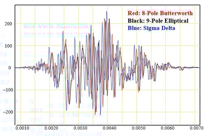
Figure 1: Pyroshock Time History Acquired With Butterworth, Elliptical, and Sigma-Delta Filters

Obviously, the results are significantly different. What can we do about this? Can we make the results acquired with one filter type look like it was acquired by another?

• • We may want to make our experimental results be compatible with others that were acquired with a different filter type, different filter setting, or different sample rate.
  • We might want to make our results look “ideal." We will see how we can remove amplitude and phase distortion introduced by the filter.
  • We may be able to increase the useful bandwidth of the acquired data.

• Resampling:
  In Blog 4 we saw that, if we use a strong anti-alias filter, the required sample rate is only slightly higher than the ideal required by Shannon’s Theorem. For instance, if we use a Sigma-Delta system, we only require the acquisition of 2.2 points/cycle of the highest frequency we care about (F_D). That certainly does not give us a very good view of the time history (Figure 2).

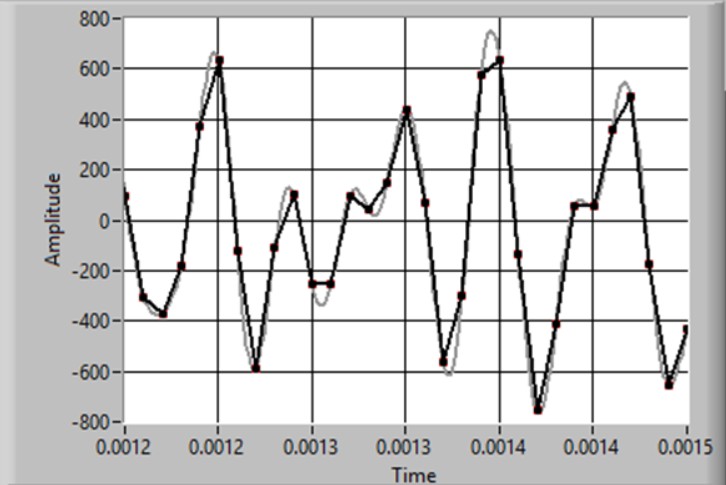
Figure 2: Sparse Time History

However, Shannon has told us that if we measure more than 2 points/cycle of the highest frequency in the signal, we know all there is to know about the signal (i.e. we can calculate as many points as we want to). (In the real world, we assume that Shannon’s theorem is satisfied if frequency components above that critical frequency are insignificant).

We also might want to change the sample rate in our test to match another one. Or we may want to mimic “synchronous” data acquisition. For rotating machinery analysis we can resample our data to provide any desired number of points per revolution of our machine.

• Integration and Differentiation: Often, we need to calculate the area under, or the rate of change, of a time series. An obvious (and commonly used) example is calculating velocity or displacement from acceleration.
• Time/Phase shift: We may want align two time histories from different tests for comparison.

There are a variety of ways to accomplish these tasks. Here we will describe spectral-domain techniques. As we will see, this approach gives us a very powerful and flexible tool set and, in some cases, a more understandable, and perhaps, more-accurate result.

Spectral-Domain Time-Series Analysis

Yes, it sounds like an oxymoron, but bear with me. Here is the basic idea:

1. Use the Fourier Transform to convert the time-domain signal to a spectrum.
2. Manipulate the spectrum.
3. Use the Inverse Fourier Transform to convert back to the time-domain.

This seems like a lot of work, but we will see that the spectral-domain approach gives us an incredibly powerful tool. In many cases, we can use the Fast Fourier Transform for our domain changes. Because it is so fast, the calculations may be quicker than their pure time-domain equivalent. In cases where the radix cannot be a power of two, most modern processors provide a very fast “brute-force” transform. With modern computers, the process is almost instantaneous.

The Basic Manipulator: The Transfer Function

The transfer function is defined as the ratio of the input and output spectra. We have used the transfer function to describe the behavior of anti-alias filters (gain and delay (phase)) as a function of frequency in earlier blogs. We treated it as a black box there. Let’s look at what’s inside the box.

First we need to make a fundamental assumption: Our system is “Linear”. Simply put, this means that if we excite the system twice as much, the response will double. Fortunately, many processes in nature (and our measurement systems) satisfy this criterion.

We have the system shown in Figure 3. The input (Drive) and output (Response) are time histories. The relation that describes the interaction is called a transfer function.

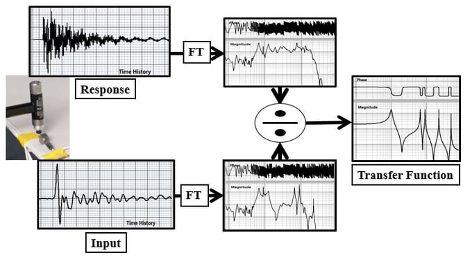
Figure 3: Transfer Function Calculation

The input can be any excitation: electrical signal generator, electrodynamic shaker, hammer, wind, earthquake…

The output might be: voltage response, acceleration, or any other reactions to the input.

The basic definition of a transfer function is:

TF = Spectrum(Response Time History)/Spectrum(Input Time History)

= Fourier Transform(Response Time History)/Fourier Transform(Input Time History)

If we move the denominator to the other side of the equal sign we get:

Fourier Transform(Response Time History)= TF x Fourier Transform(Input Time History)

Taking the inverse transform of both sides we get

Response Time History = Fourier Transform ^-1(TF x Fourier Transform(Input Time History))

So, if we know the Transfer Function and the Input Time History, we can calculate the Response Time History (Figure 4).

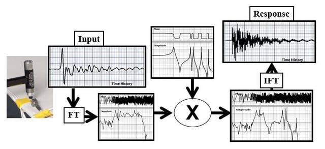
Figure 4: Spectral-Domain Time-Series Processing

So, now we have the tool necessary to do filtering in our analysis. And, we can make the filter any shape we want. Earlier, we looked at Bessel, Butterworth, Elliptical, and Sigma-Delta filter transfer functions (Figure 5).

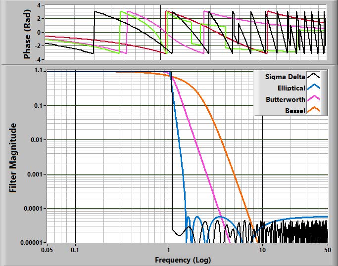
Figure 5: Filter Spectral Shapes and Phases

I made the time histories shown in Figure 1 using 10 KHz filters of each filter type on a pyro-shock time history.

So, what can we do with it other than this straightforward filtering operation?

Using the spectral-domain approach allows me to easily design and use a filter that has any shape. For instance, if I have a 60 Hz noise problem, I can notch it out (Figure 6).

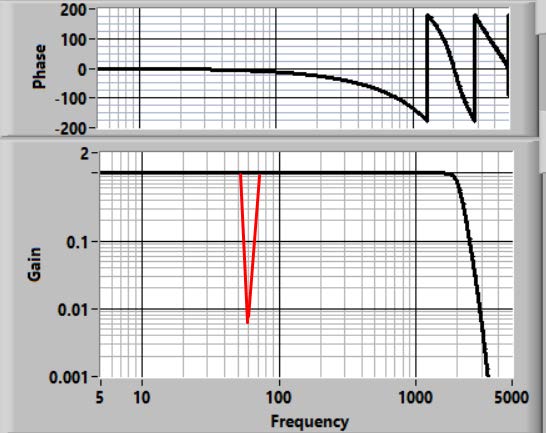
Figure 6: Notch Filter

In principle, with the caveats to be covered shortly, we can use an etch-a-sketch approach to build a filter with any amplitude and phase characteristic.

But, let’s get practical (more useful?).

Filter Transfer Function “Correction”

Let’s say that our data acquisition system hardware has a 5-pole Butterworth filter and we don’t like the resulting attenuation and phase-shift characteristics. Can we make the result look like the filter we want?

Maybe we like an 8-pole Butterworth filter better (or maybe we want to match another investigator's results where an 8-pole filter was used).

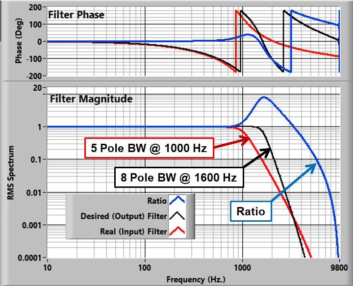
Figure 7: "Correction Filter"

The process is to make up a filter (transfer function) that “backs out” the real filter and applies the desired one. One of the magic features of transfer functions is that this is a simple division of the respective individual transfer functions. Figure 7 shows the “filter” that results from dividing an 8-pole, 1600 Hz Butterworth by a 5-pole, 1000 Hz. Butterworth filter.

You can see that the new (“correction”) filter produces gain above the cutoff of the denominator filter. At 1600 Hz, the gain is about 8.

Why did I choose 1600 Hz. for the “desired” filter cutoff? This is an engineering decision that is dependent both on the desired response and on the noise in the signal. The gain of the correction filter will be applied to the original measured signal. Whether it will work properly depends on the high-frequency signal-to-noise ratio of the experiment.

Let’s do a “real” example.

Let’s apply this strategy to data acquired with an Endaq Slam Stick X. I have made a very simple experiment that applies a sharp, very repeatable, shock to the transducer. Figure 8 shows the setup.

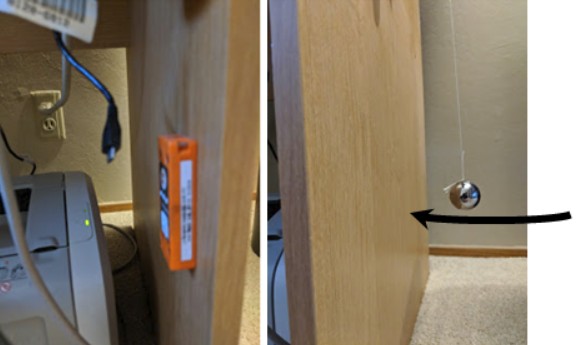
Figure 8: The Experimental Setup

• The Slam Stick is attached to my desk leg with the provided double-sticky-side tape.
• Excitation is provided with a pendulum weight that uses a ¾ inch ball bearing as an impactor.

The Slam Stick is set up with the following characteristics:

• Sample Rate: 20 KS/S (the maximum)
• Anti-alias filter (5-pole Butterworth (Hardware)) cutoff: 5 KHz. (the default).
• The time history and RMS spectrum are shown in Figure 9.

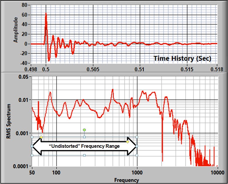
Figure 9: "Broadband/Reference" Signal

• The signal looks good/reasonable. The energy is well-rolled-off above 8 KHz. Well below the Nyquist Frequency, indicating good alias rejection.
• For the purposes of this discussion, we will assume that the filter response is flat and the phase response is linear from zero to 1000 Hz… i.e. the response is insignificantly distorted. (See discussion of Butterworth filters in Blog 4). We will call it the “Broadband Signal."

Next, we repeated the experiment but with the 5-pole filter set to 1000 Hz. Figure 10 shows the resulting time history and spectrum.

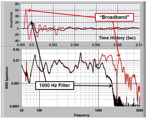
Figure 10: “Broadband” and Filtered Response

Our objective is to make the data look like it was acquired with an 8-pole, 1400 Hz. Butterworth filter. To do this, we apply the correction filter developed earlier. The result, overlaid with the result of analytically filtering the “broadband” data with a 1000 Hz. 8-pole filter, is shown in Figure 11. They agree very well.

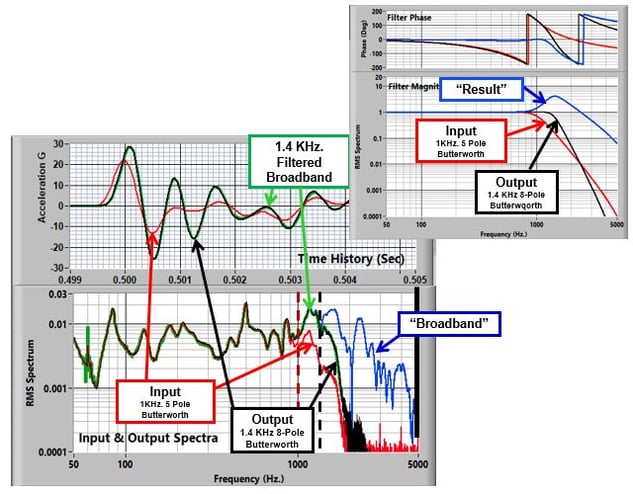
Figure 11: Butterworth "Adjustment" Results Overlaid

The agreement (Green (real filter)-Black(“corrected”)) is excellent as seen in both the time and spectral plots.

The “correction” has produced a time history whose bandwidth is increased by a factor of 1.6. The energy is increased by a factor of 2.05 and the peak response has increased from 23.3 G to 30.4 G. This is because of two factors:

• including more energy and
• a change in the phase characteristics.

Next, let’s push the concept to the next level.

In the earlier blogs, I discussed the concept of analyzing the data over a bandwidth of zero to F_D. The objective is to get minimally-distorted data within that frequency range and reject all energy above it. This requires a very-sharp filter that might be supplied in real life by an elliptical analog or sigma-delta hybrid system.

In this “analytical” world, we can build a “perfect” filter: One with “square” amplitude characteristics and zero delay. Use of this filter allows us to move the output filter out to 1700 Hz. before there is too much noise interference. The result is shown in Figure 12).

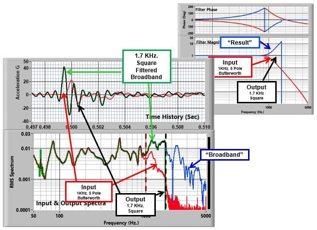
Figure 12: Square Filter "Adjustment" Result Overlay

The output of the 1KHz. filter has been modified to have:

• Ideal gain characteristics out to 1700 Hz.
• Zero phase/delay. The Butterworth delay characteristics (and phase non-linearity) have been backed out.

This combination backs out the characteristics of the real filter.

In addition, there is response ahead of the main pulse. This cannot happen in the real world. This effect is called Gibb’s Phenomenon and it happens when a spectrum is truncated abruptly (as is the case here).

It looks a lot like what we saw in Blog 6 where we discussed Sigma Delta ΣΔ data acquisition systems. The real ΣΔ system has a very similar (but not quite as sharp) filter cutoff and large delay.

Is this a better representation of the acquired signal? It is certainly more “pure”.

Integration and Differentiation

Integration and differentiation are normally done in the time domain using classical techniques such as Simpson’s rule. However, as we will show, the processes can also be done in the spectral domain and the results are more accurate. An additional advantage is that viewing the process in the spectrum can give us a better understanding of the operations and their consequences.

The equations for, and a graph showing the gain of integration and differentiation of a sine wave, are shown in Figure 13:

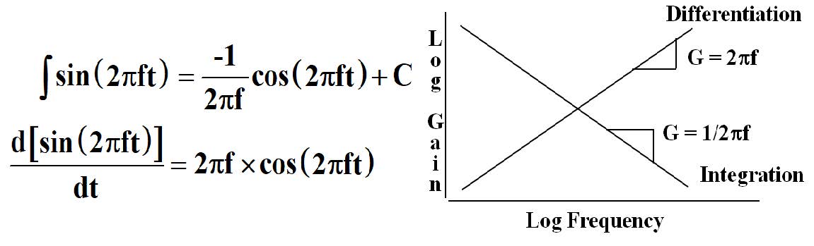
Figure 13: Integration and Differentiation Gains

Integration produces a gain inversely proportional to frequency and a phase lag of 90°. Differentiation has gain proportional to frequency and phase lead of 90°.

What we see from the plots is:

• For integration, the gain at low frequency is very high. In fact, it is infinite at zero frequency. Hence, low frequency experimental errors will be amplified. A common usage of integration is to calculate velocity and displacement from acceleration measurements. Small errors at low frequency can cause huge errors in velocity and displacement results.
• For differentiation, the gain at high frequency is very high. High frequency noise will be amplified.

A very simple example of spectral integration is shown in Figure 14. As you can see, low-frequency signals are increased and high frequencies are attenuated.

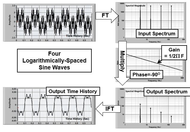
Figure 14: Integration of Sine Waves

Spectral integration and Simpson’s rule on our shock time history are shown in Figure 15.

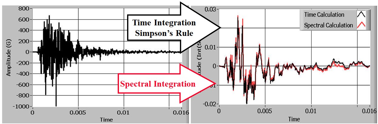
Figure 15: Integration by Spectral Calculation and Simpson's Rule

We see that there is a pretty significant difference. In particular, it looks like the high-frequency peaks have been attenuated. When we look at the transfer function of Simpson’s Rule we see that it actually forms a low-pass filter in addition to integration. There is an attenuation of 10% at 0.15xS and the attenuation approached 50% at the Nyquist Frequency (S/2).

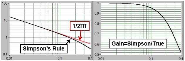
Figure 16: Comparison of Spectral Domain and Simpson's Rule Integration

The result is that for frequency components below S/10 Simpson’s Rule works well. For signals that have frequency components above S/10, the spectral approach is superior.

One obvious problem with spectral integration is that the gain at zero frequency is infinite. Therefore, any dc component of the signal will blow up. The solution is to:

1. Zero the zero-frequency element of the integration transfer function.
2. Calculate the mean and subtract it from the time-series input.
3. Integrate the result using the spectral approach.
4. Calculate the time history of the integral of the offset = offset x time.
5. Add this slope to the calculated integral.

An additional advantages of the spectral approach is that, once we recognize that the processes are actually filters, we can modify the transfer function to suite our needs. Multiplying the basic integration transfer with the desired high- or lowpass filter characteristic will produce the desired results (Figure 17).

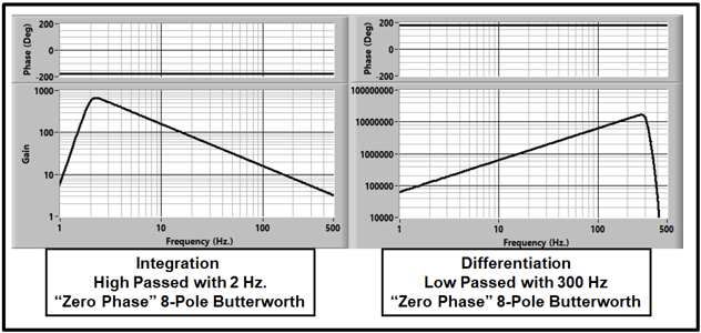
Figure 17: High-Passed Integration and Low-Passed Differentiation

Time/Phase Shifting

When we are comparing time histories from two different tests we might want to time-align them to enhance comparison.

“Rough” alignment is done by simply shifting one time series by an integer number of points. If finer alignment is needed it can be done in the spectral domain with a transfer function that has unity gain and a constant phase shift of the desired amount (Figure 18).

The time delay will be (Phase(deg)/360)/(Sample Rate). The phase lies between + 180 degrees (+1/2 cycle).

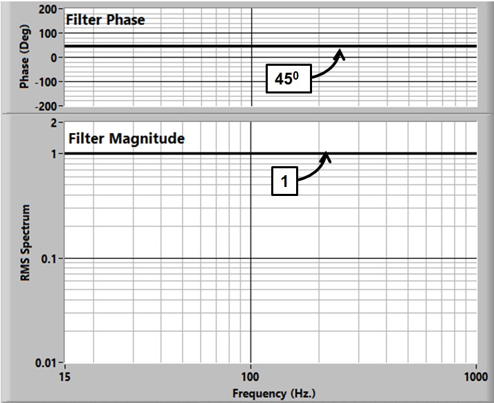
Figure 18: 45 Degree Phase Shift Spectrum

Resampling

One of the coolest things about spectral-domain time-series analysis is that you can manufacture data out of thin air.

As we mentioned earlier, if we satisfy Shannon’s theorem, we know all about the time history. The challenge is to figure out how to calculate more points than the original time series.

There are a variety of strategies that have been used such as spline and polynomial-curve fitting. These are approximate but work well when the initial point density is high. The strategy discussed here is exact (to the limits of the arithmetic used).

It uses the spectral approach.

First, we need to understand a few of the basic operations of the discrete Fourier Transform:

If we acquire N points in our T seconds-long input time history (Sample Rate=S=N/S), the Fourier transform will produce N/2 unique complex values (or magnitude/phase points) between 0 and the Nyquist frequency (F_N=S/2) (Figure 19).

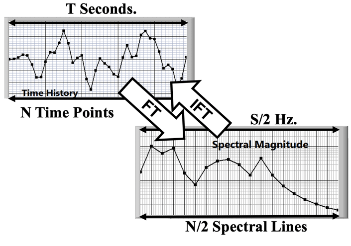
Figure 19: Fourier Transform Basic Properties

Figure 20 shows a cartoon of the spectral-domain Upsampling process. The operations are:

• Calculate the Fourier Spectrum of our data.
• Add zeroes to the top of the spectrum (padding).
  • This adds to the number of points but does not change the data in any way.
• We do the inverse Fourier Transform.
  • Since there are more points in the spectrum, there are more points in the time history.
  • They are equally spaced between zero time and T.

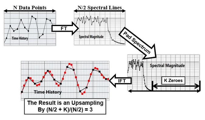
Figure 20: Upsampling Process

Let’s look at a real example. We will use our impact experiment data and filter it with a very sharp filter set at 1 kHz. We then decimate it down to 2500 S/S to produce a sparse, but unaliased time history (Figure 21, upper frame, black line).

We calculate the spectrum of the 3,750 point time history to produce a spectrum with 1875 unique points. We pad the spectrum with 13125 points to produce a total of 15,000 points. We do the inverse transform to produce the upsampled, 15,000 point time history (Red curve in Figure 21).

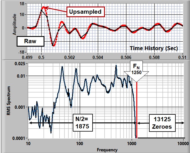
Figure 21: Upsampling Example

So, how many points/cycle do we need to get a good representation of the time history? If we assume the worst case: Acquired points are equidistant from the peak, we get:

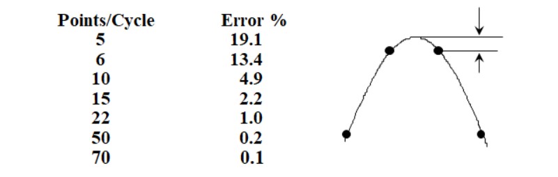
So, if we want to guaranteeing finding the peak within 1%, we need to have at least 22 points/cycle at the frequency of the component.

Normally we upsample by an integer ratio (8 in this case) but it is important to note that we can pad with any number of zeroes so that the upsample ratio is essentially arbitrary.

There are at least two instances where a non-integer sample ratio might be used:

• Compare two tests that have been run at different sample rates. If they are acquired at 1000 S/S and 1024 S/S, the slower one can be upsampled by 1024/1000.
• In rotating machinery applications, it is often required to sample with a constant number of points per revolution. Data from a constant-sample-rate acquisition system can be resampled based on the tachometer signal.

Downsampling

Sometimes we have a data set that is acquired at a rate that is much higher than required. You can reduce the sample rate by an essentially arbitrary amount by using the opposite approach: removing points from the spectrum.

For instance, the 1KHz. filtered data in Figure 10 shows that the signal spectrum is down to the noise floor at about 2,500 Hz. So, we can reduce the sample rate to 5KS/S without affecting the real part of the signal (Figure 22).

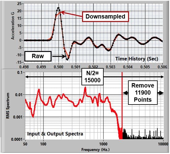
Figure 22: Downsampled Time History

However, we have obviously hurt the time-domain representation.

If we are only interested in data to a lower frequency, we can downsample further. The spectral downsampling process produces a “square” filter at the Nyquist frequency. In Figure 23 we see the results of downsampling by a factor of

Again, we see the effects of cutting the spectrum off sharply. There is ringing before the shock due to Gibb’s phenomenon.

Is it useful to resample by a non-integer factor? That depends on the application, but performing it in the spectral domain allows any ratio whose denominator is the (number of points in the time history)/2.

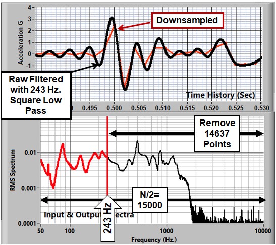
Figure 23: Downsampling by 41.3

Combining the Functions

We have demonstrated a general-purpose algorithm that:

1. Filters the data with an etch-a-sketch spectral shape and phase
2. Allows modification of the data to make it appear like it was acquired with a different anti-alias filter (including the option of a perfect (square, zero-phase) characteristic)
3. Integration and Differentiation
4. Time/Phase shifting
5. Resampling to provide up/down sampling of the time history data with an essentially-arbitrary resample ratio

…for any time history.

These operations are all performed in the spectral domain using transfer functions. These transfer functions can be combined by multiplication to build a total “filter” to calculate the time history and spectra of the combined effects.

Let’s start with the enDAQ data acquired at 20,000 samples/second with a 300Hz, 5 pole Butterworth filter. The bandwidth of the signal is about 600 Hz so we can safely decimate it down to a sample rate of 2000 S/S. However, this makes the time history too sparse to determine peaks accurately.

Now lets apply the following adjustments:

• Make the data look like it was acquired with an 8-pole Butterworth filter at 500 Hz.
• Integrate it once to velocity (Velocity is often considered to be a better criterion for damage than acceleration)
• Upsample the data by a factor of 2.314 to improve peak detection. (We are using a non-integer upsample ratio just to prove we can.)

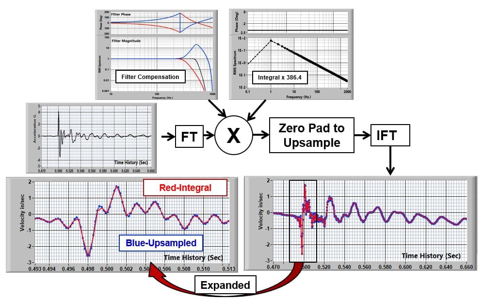
Figure 24: Combining Operations

But We Have Cheated…a Little….No, a Lot

Practitioners of the signal processing art will note that my examples have all been transients: Signals that begin and end quiescently and near the same level.

Because Fourier Theory assumes that our signal is infinitely long, and we can only handle a small block in our processing, this process falls apart for continuous signals like random. For transients, we assume that the signal is repeating but this is not the general case. For continuous signals, we have to use another tool.

“Fast Convolution” to the Rescue

Convolution, briefly discussed in Blog 6, is a very computationally intensive method of performing time domain filtering and resampling. Researchers discovered that, because of the efficiency of the Fast Fourier Transform, the convolution could be done much faster by transforming to the spectral domain, manipulating the spectrum, and then transforming back... exactly the process we have described here. But, they had to come up with a means to get around the Fourier-Transform shortcoming. They came up with the concept of windowed, block overlapped processing.

The process for handling arbitrary signals is:

1. The time history is broken down into 50% overlapping blocks. The length is arbitrary but, if you want to take advantage of the speed of the Fast Fourier Transform, it should be a power of two (2^N).
2. Each block is multiplied by an offset cosine (Hanning window) (Figure 25).

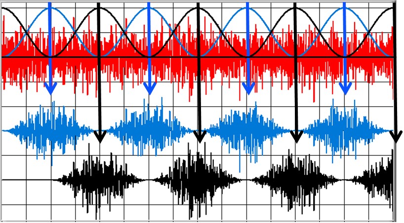
Figure 25: Overlapped and Windowed Time History Blocks

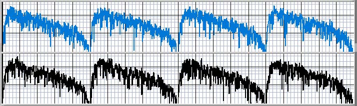
Figure 26: Spectra of Windowed Blocks

4. Each block’s spectrum is multiplied by the filter transfer function and padded/reduced for up/down sampling to calculate the output spectrum (Figure 27).

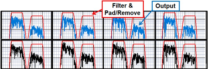
Figure 27: Filtered/Padded Output Spectra

5. The time history of each windowed/manipulated block is calculated with the inverse Fourier Transform and the overlapped blocks are added to produce the output time history. (Figure 28)

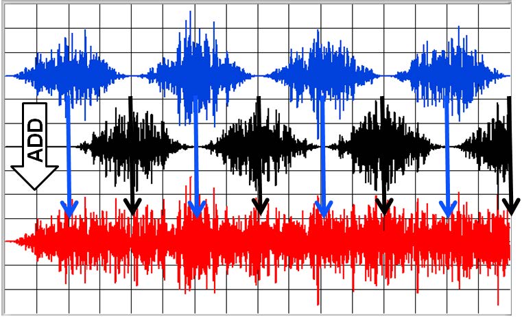
Figure 28: Inverse Fourier Transform of Each Block and Summing

This seems like a lot of work and it is, but that is what computers are for. It goes very quickly with a modern PC.

Note that the first and last half blocks still have the shape of the window. This part of the data is distorted and should be thrown away.

Conclusion

The concepts presented here give the investigator a powerful set of tools to manipulate the data. The objectives are to correct for some of the shortcomings in the data acquisition process.

The tools modify the results that are acquired with a “perfect” data system to make them look like they were measured with a different “perfect” system. We can perform operations on the data to make it look like it was acquired with any system that has the same bandwidth or less.

We have paid a lot of attention to compensating for the effects of the anti-alias filter. It is required that we have a filter because, if the data is not adequately alias-protected, there is no data manipulation that will produce good results.

Are the results produced by these manipulations a better representation of the “truth” than the raw data? Does a square, zero-phase filter produce a better representation than a 5-pole Bessel system?

These are questions that you must answer yourself. Earlier blogs have discussed the pros and cons of different analog filter strategies. The tools presented here allow the user to make the data look like it was acquired with a different analog filter... or, for that matter, with a filter of any shape. Are there advantages to doing this. That is the user’s option.

Your comments are solicited.

Send a Comment or Question to Strether

One of the reasons I've been writing these blogs is to get a discussion going. Please reach out to me with any questions or comments you may have.  

You can participate by:

• Entering comments/questions below in the Comments Section at the end of the blog. This will obviously be public to all readers.
• Contact me directly. I will respond privately and (hopefully) promptly. If appropriate, your question could be the subject of a future blog.

This blog is meant to be a seminar... not a lecture. I need your help & feedback to make it good!

Additional Resources

If you'd like to learn a little more about various aspects in shock and vibration testing and analysis, download our free Shock & Vibration Testing Overview eBook.  In there are some examples, background, and a ton of links to where you can learn more. And as always, don't hesitate to reach out to us if you have any questions!

References

Transfer Function Correction:

Strether Smith and William Hollowell, Techniques for the Normalization of Shock Data, Proceedings of the 62nd Shock and Vibration Symposium (October 1991) [PDF Download]

Resampling:

Strether Smith The Interpolation of Sparse Time History Data, Proceedings of the 65^th Shock and Vibration Symposium (October 1994). [PDF Download]

https://en.wikipedia.org/wiki/Upsampling

Applying the Inverse FFT for Filtering, Transient Details and Resampling,
Howard A. Gaberson; Sound and Vibration Magazine, August 2005

Fast Convolution:

The Scientist and Engineer's Guide to Digital Signal Processing

Prosig:

The Prosig Blog has several discussions about spectral calculations (that they call "Omega Arithmetic)

Shock Response Spectra Analysis

Strether Smith and Bill Hollowell:  A Proposed Method to Standardize Shock Response Spectra (SRS) Analysis: May/June 1996 Journal of the Institute of Environmental Sciences [PDF Download]

Disclaimer:

Strether has no official connection to Mide or enDAQ, a product line of Mide, and does not endorse Mide’s, or any other vendor’s, product unless it is expressly discussed in his blog posts.