Reducing Measurement System Distortions with Transfer Function Correction Strategies

Transfer Function Correction Strategies For Reducing Measurement System  Distortions

In the previous eleven blogs I have discussed many of the pitfalls that you might encounter when measuring data from your experiment. Here, I will tackle strategies to correct for distortion that is caused by non-idealities in the measurement chain components.

Topics covered include:

1. Our Measurements: Fact or Fiction
2. Transfer Functions: A Few Basics
3. The Transfer-Function- Correction Process
4. The Data Acquisition Process
5. Where Do the Transfer Functions Come From?
6. Experimental Determination of the Data System Transfer Function
7. The System Transfer Function
8. Transfer Function Compensation
9. How Much Can You Increase the Bandwidth??
10. UpSampling
11. Conclusions and Caveats

Our Measurements: Fact or Fiction?

Our measurement systems lie to us. At best, they give us a distorted vision of the truth. In the first blog Is Your Data Acquisition System Telling You the Truth? I discussed the fact that a measurement system is a lot like your favorite news source (Figure 1). There is a process that occurs between the truth and what gets reported. In news terms, it’s called “spin”. In the measurement world, it’s called distortion. In both cases, the result is, almost certainly, not the real truth.

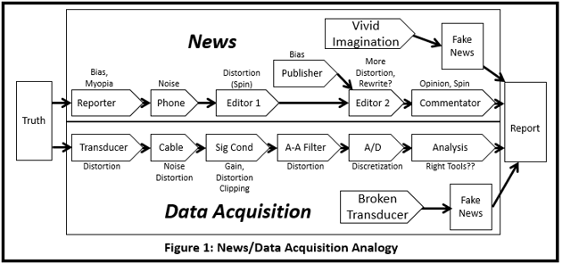
In that discussion, we briefly looked at the effect that physical devices and physics have on the measured data. The conclusion there was that different “correct” systems and data acquisition strategies will produce different results. Here, we will continue the discussion and describe techniques that might:

• Reduce the effects of the distortions.
• Standardize the results between different tests and facilities.
• Increase the time resolution to give a better representation of the peaks and other time-domain details.
• Extend the accurate frequency range of the measurement to beyond the nominal measurement bandwidth of the system.

In the corrections we will be describing there are key assumptions and limitations:

• We assume that the measurement system components respond linearly.
• We can only compensate for known and modellable errors.
• The methods we are describing do not address zero-shift, thermal transients, EMI and/or off-axis induced distortions, base strain distortions, or any nonlinearities.

The tools required to accomplish these goals were discussed in my earlier blog: Spectral-Domain Time-Series Analysis. Here we will use them to apply them to the tasks listed above.

Transfer Functions: A Few Basics         

The fundamental tools that we need to accomplish these goals are the Fourier Transform and the Transfer Function.

The Fourier Transform was discussed in Steve Hanly's earlier blog. Here we will treat it as a black box that converts time histories into their frequency-domain representation. The basic properties of the transformation are shown in Figure 2.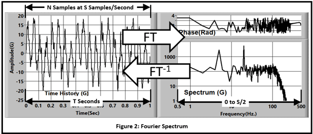

The calculation is reversible: We use the forward transform (FT) to go from time history to spectrum and the inverse transform (FT^-1) to go in the opposite direction.

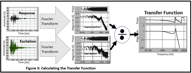
The Transfer Function is calculated by dividing the spectrum of a response by the spectrum of an input (Figure 3). This gives us a spectral representation of the phase (delay) and the magnitude ratio between two signals as a function of frequency.

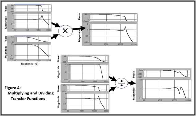
Transfer functions can be multiplied and divided like ordinary numbers using complex math with real and imaginary components (Figure 4).

While we are in the spectral domain, we can also increase the time resolution by adding zeroes to the spectrum. (Figure 5).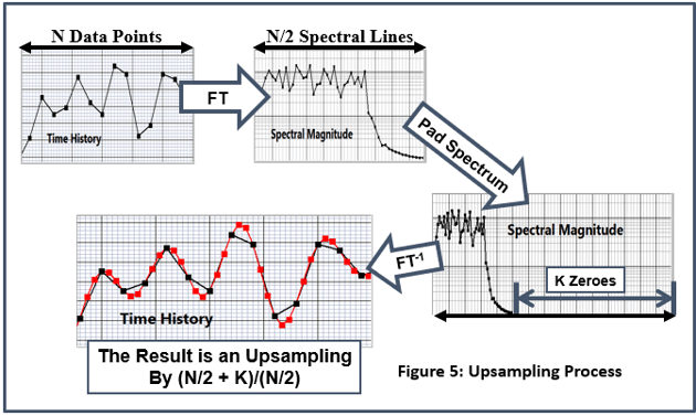

Spectrum modification (Figure 6) uses a calculated transfer function to modify the frequency content and produce a new time history. This is called Forced Response Analysis.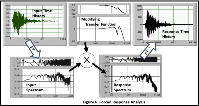  

We will use all of these functions in this discussion.

The Transfer-Function-Correction Process

Figure 7 shows all of the steps in the data acquisition and data correction/enhancement process. There are three sections:

• Truth->Measured: The Truth at the specimen is what really occurs and is never really known. This response is passed through the measurement system to produce the measured signal. The measured signal contains a combination of the Truth and the Distortion. Its Spectrum is calculated by a Fourier Transform (FT).

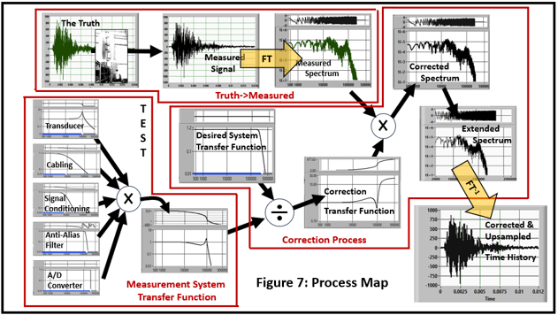
• Correction Process: The “Corrected and Extended Spectrum” is calculated by:
  • A Desired System Transfer Function is selected. This can be any characteristic but likely candidates are:
    • Constant Amplitude to a cutoff frequency and zero phase (An “ideal” Result, Shown).
    • Matching results from another system using the known transfer function of that system.
    • Matching “Standard Results”.
  • The Correction Transfer Function is calculated by dividing the Desired System TF by the Measurement System TF.
  • The Measured Spectrum is multiplied by the Correction Spectrum.
  • The Extended Spectrum is created by “padding” the Corrected Spectrum with zeros.
  • The Inverse Fourier Transform (FT^-1) calculates the Corrected and Upsampled Time History.
    
    

The Data Acquisition Process

A typical vibration/shock measurement system looks like Figure 8. It is made up of:

• The transducer that converts a physical input into an electrical signal. Its characteristics may include:
  • Transducer resonance.
  • Frequency/band limiting/filtering due to inherent physical and electrical limitations.
  • Transducer mounting blocks may produce a low-pass-filter effect.
• The cable will act as a low-pass filter due to transducer output impedance and cable capacitance (Reference 2), interaction with the transducer (Reference 3), or a number of other issues.

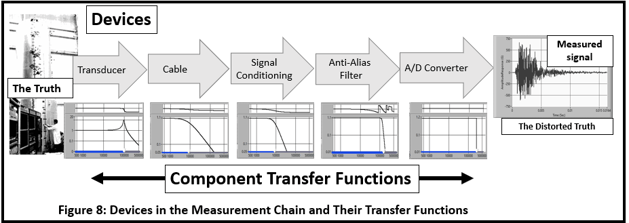
• The signal conditioner, that further processes the analog signal, may appear as both a high- and low-pass filter.
• The analog anti-alias filter, required for any digital data acquisition system, will distort the amplitude and phase characteristics and limit the useable frequency range.

The A/D converter will limit the bandwidth of the measurement to the Sample Rate/2. It will also limit the time resolution to ∆t=1/Sample Rate. This may not give enough time points to adequately describe the time history.

Where Do The Transfer Functions Come From?

 We Need to Understand How Each Device Works.

Each of the components in the measurement chain contributes to distortion. Some of them, like the analog filter protecting our data from aliasing, are necessary. Others, like the resonance of a piezoelectric or piezoresistive accelerometer or the inherent roll-off of a signal conditioner, are a consequence of the technology used. In any case, every component in the instrumentation train causes distortion…some large, some small; none are zero.

The measurement system manufacturers have gone to great lengths to produce devices/components that reproduce the phenomena that they are measuring as accurately as possible. However, at some frequency, their response deviates from the ideal. This is normally used as the limit of the usable frequency range. However, if the transfer function is known, the useable frequency range may be extended.

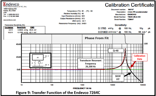
For instance, the Endevco 7264C piezoresistive vibration/shock accelerometer has the frequency response shown in Figure 9. The calibration curve (black) is closely matched by the overlaid characteristic of a classic SDOF mode model (red). The accelerometer is normally used with a frequency range of 5KHz, where the gain deviation is small. However, since we have a good characterization of its transfer function, the usable range can be expanded to a much higher frequency…perhaps up to 20KHz with small error. In addition, the analytical representation (fit) also provides the phase information needed to correct for the transducer signal delays. (Thanks to the folks at Endevco and PCB for providing the extended-frequency-range calibration curve).

Next, the high output impedance of this accelerometer, when combined with the resistance and capacitance of long instrumentation cables, will act as a one-pole low pass filter.

Using the analysis approach of Reference 2 we can calculate the filter cutoff for 200 feet of PCB #96 cable to be about 7.6 KHz.

This one-pole-filter behavior appears in many data measurement systems (Figure 10). It is particularly troublesome because of its significant attenuation characteristic below the nominal cutoff frequency. At ½ of the cutoff frequency, the attenuation is 10.4%. The attenuation is greater than 1% above 0.18 x F_C.

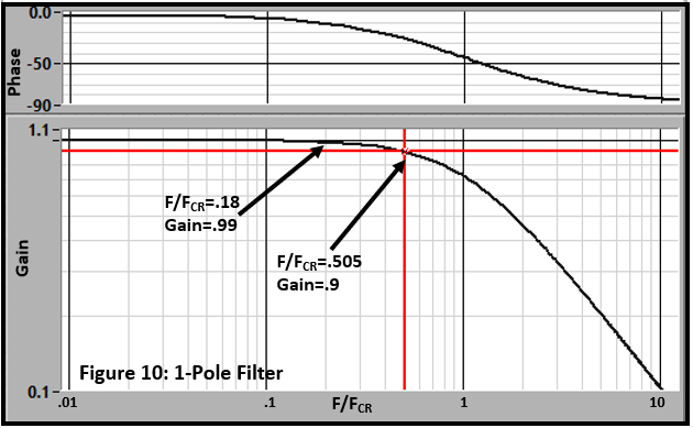
(Anyone that thinks they are acquiring data to an accuracy of 1% should pay close attention.)

All digital data acquisition systems require an analog low-pass filter before digitization to reduce high-frequency energy that causes aliasing. Conventional converters (SAR) require “significant” conditioning such as Butterworth or elliptical filters that will contribute substantial distortion.

Properly implemented Sigma Delta (or oversampling) converters offer a very-nearly perfect constant-amplitude, constant-delay transfer function to about 45% of the sample rate. However, a very good analog filter ahead of it is required to come close to a “nearly perfect” result.

Our objective is to characterize, and compensate for, their distortions.

Experimental Determination of the Data System Transfer Function

The behavior of all of the components in the signal train beyond the transducer can be determined experimentally. A sine-wave generator and a system-response readout/recorder can be used to generate a characterization of the amplitude of the transfer function (Figure 11).

The transducer is replaced with an emulation of its output impedance.

• IEPE Devices: A Resistor
• Bridge devices: Use the device with zero excitation.
• Charge devices: a capacitor.
• Many devices can be characterized by simply isolating them from the environment. An example is putting an accelerometer on a pillow. This is the best approach for devices that can be isolated.

Set the data acquisition system up with the parameters (gain, filter cutoff, sample rate...) that you normally use.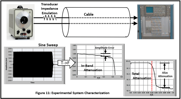

First, a data set should be acquired to determine the “zero-input” noise level. Acquire a 10 second record and calculate its RMS and Fourier Spectrum. This will produce a baseline for future use and point out any spectral components that might need attention/correction in the experiment.

The simplest thing to do is perform a manually stepped frequency “sweep” taking measurements from low frequency to the sample rate (or higher). A smooth curve is passed through the acquired frequency/amplitude data set. Measure both the RMS and DC values. The oscillating amplitude should roll off as the Nyquist Frequency (Sample Rate/2) is approached. The response should be very small at high frequency.

A better characterization can be done with a continuous sweep generator that is analyzed with a sine frequency/amplitude processor. The amplitude transfer function of the system plot is characterized by the two views shown in Figure 11:

• In-Band Amplitude Error: An expanded vertical scale plot of the attenuation from low frequency to the Sample Rate/2 (Nyquist Frequency).
• Total Attenuation: The full amplitude range plotted from low frequency to the maximum of the sweep range.

These characteristics will define the fundamental accuracy in the frequency range of interest and the rejection of out-of-band (aliasing) signals.

The System Transfer Function

The system or component transfer functions are multiplied together to calculate the System Transfer Function (Figure 12).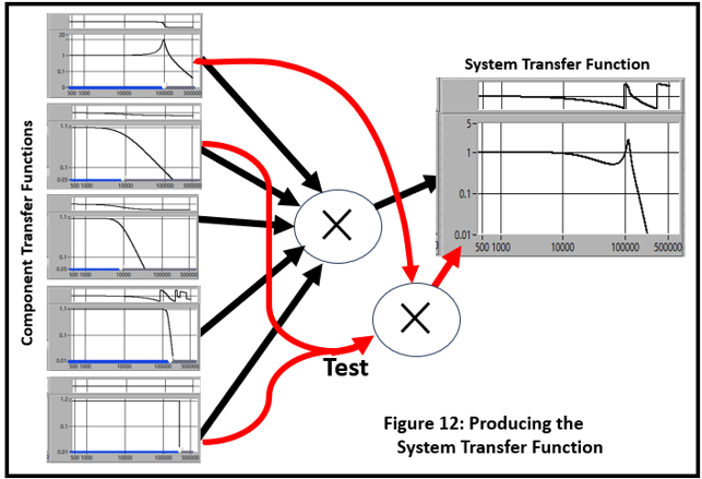

The “Desired System Transfer Function”

The objective of the procedure is to make the results look like they were acquired with a data system that has a particular “standard” transfer function. There are two obvious possibilities:

• Matching a different system’s transfer function. For example, data acquired with a sigma-delta system can be made to look like it was measured with a Butterworth filter.
• An “ideal” transfer function: Constant gain and zero phase to the cutoff frequency. Zero response above it.

There are restrictions to the selection of the Desired Transfer Function. The gain must:

• Roll off faster than the system transfer function.
• Not amplify noise “excessively”.

Compromises are required.

Transfer Function Compensation

For an example, we will build a fairly extreme “system” so that the changes will be obvious.

Our model measurement system has the following characteristics:

• The nominal system bandwidth is 10KHz.
• The transducer has a resonance with a Q of 10 at 8KHz.
• The cabling system and signal conditioning act as a 1-pole low-pass filter at 2KHz.
• The anti-alias filter is a 4-Pole Bessel Filter at 10KHz.

We will use a shock acquired at 100KS/Sec as the “true” input time history.

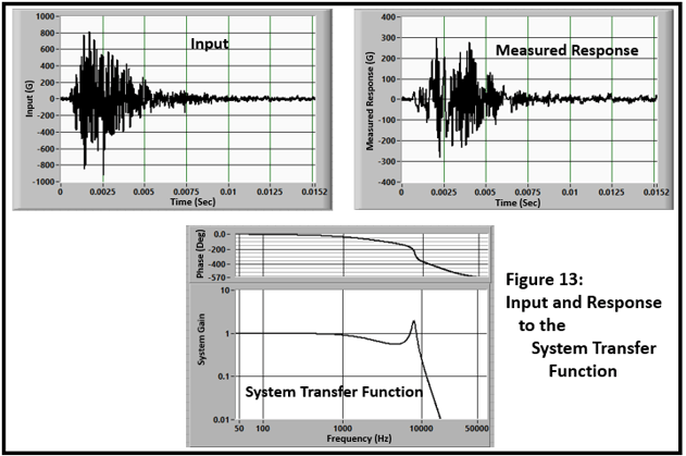
The input time history, system transfer function, and measured response are shown in Figure 13. The system has attenuated the energy at high frequency and modified the level significantly.

Our first objective is to emulate a system with zero phase (delay) and a flat spectrum with a bandwidth set to the nominal value of 10KHz (Figure 14).

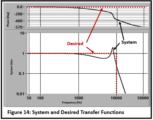Figure 15 shows the result of the correction. The “Corrected Response” is essentially identical to the input processed with the “ideal” low-pass filter.

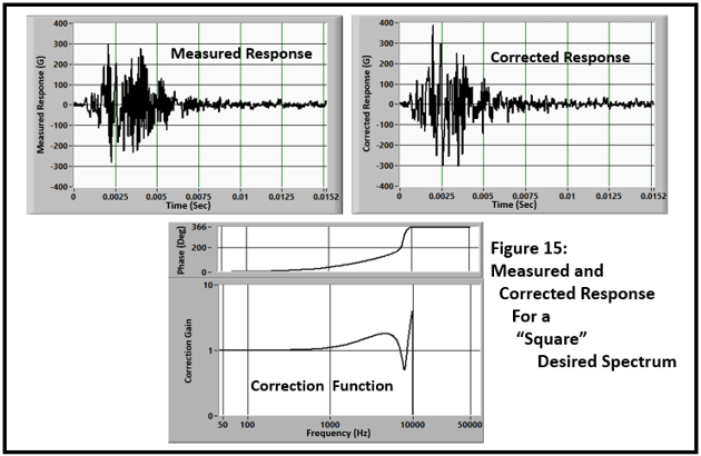
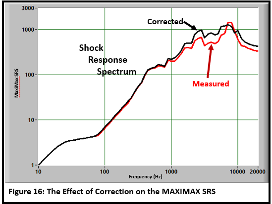
Figure 16 shows the effect on the Shock Response Spectrum: an increase of about 70% at 5KHz.

How Much Can You Increase the Bandwidth?

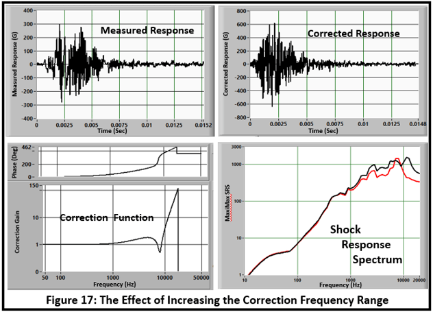
In theory, you should be able to expand the frequency range up to the Nyquist frequency. However, the correction at high frequency gets large because the roll-off of the Desired Transfer Function must be steeper than the system characteristic and the result is multiplied by the system noise. The input-noise test recommended above will provide information required to determine the signal-to-noise ratio. Realistically, with a good 16-bit (or more) data system the signal-to-noise ratio should be at least 1000/1 so it is reasonable to allow a correction gain of 100. For this example, the square-filter cutoff can be increased to 17KHz (Figure 17). The time history magnitude is significantly increased but the effect on the SRS is negligible.

Significant art and engineering judgement is required.

UpSampling

Finally, if there is not enough resolution in the time-domain representation, the signal can be upsampled by adding zeroes to the top of the spectrum before converting back to the time domain as shown in Figure 5.

Conclusions and Caveats

The measurement system that we use produces distortions that can be defined by transfer functions. These distortions can be compensated to produce a data set that has a “standard” characteristic provided that our structure and measurement system satisfy the assumptions and limitations stated near the beginning of this blog.

For non-transient signals the processes described here must be generalized to use the overlapped/windowed approach described in the earlier blog: Spectral-Domain Time-Series Analysis.

References

1. Enhancing Signal Accuracy and Bandwidth Extension in Transient Shock Measurements Using Transfer Function Compensation Strether Smith and Ted Diehl. 93^rd Shock and Vibration Symposium, October 2023.
2. MEMS Shock Accelerometer Signal Modification Attributable to The Electrical Impedance Of Their Cables Patrick Walter, Alan Szary, James Woernley 2021
3. Driving Long Cables PCB TN-7