The process of digital data acquisition has been the subject of hundreds, if not thousands, of books, papers, and theses since its rise to usefulness in the 1960s. Here is yet another.
I will examine the "accepted" approaches to the acquisition/quantizing process and offer a new one that I think is better. To do this, we need to look at:
- Sampling and Quantizing Basics
- The Classic Quantification Derivation
- A Simpler View of the Classic Derivation
- Modeling the Process
- The "Shannon View" of the Process
- Analyzing the Signals Using "Shannon's View"
- The Strange Relationship: SNR(dB) (or RNR(dB) = 6.02 N + 1.76 (dB)
- Conclusion
Sampling and Quantizing Basics
The digital data acquisition process is made up of two stages:
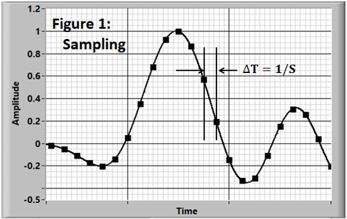
Sampling, where a “snapshot” of the input signal is taken at a series of time points (Figure 1). Normally, the samples are taken at a constant time spacing ΔT = 1/Sample Rate.
Next, the sample is quantized (Figure 2).
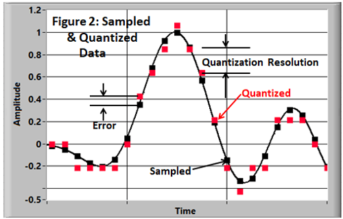
The quantization process “rounds” the sample to the nearest resolution point of the measurement system. The difference between the sample and the quantized version is the error.
For a binary system (the most common), the quantization increment (resolution) is defined by the number of bits:
Resolution=Range/2N
so Resolution/Range = 1/2N (1)
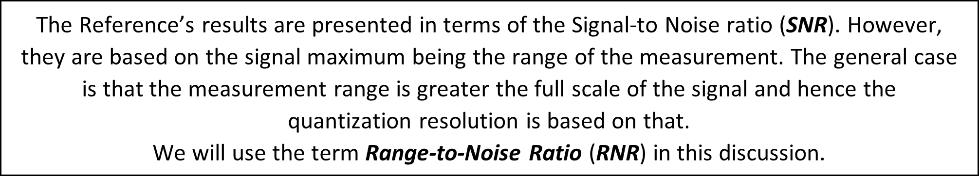
|
The terms Digitization, Discretization, and Quantification are all used to describe the resolution of the signal’s amplitude into discrete elements. We will follow the example of References 1 and 2 and use the terms: |
The Classic Quantification Derivation
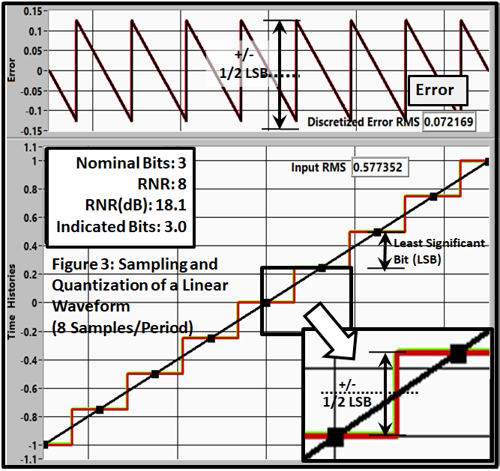
The generally accepted derivation of the error due to the quantization process is presented in References 1 and 2. The model used in their derivation is shown in Figure 3. It shows the quantization of a +/-1 unit straight line wave sampled with 3-bit (8- step) conversion. The sample rate (8 points/period) is the number of steps (2N=8) required to properly synchronize the process.
Each sample (black squares) is pictured as a constant value between +1/2 sample (red line). Each step is 1 LSB high and the measurement will fall within +1/2 LSB of the truth.
Their derivation produced the result (with a modification to be discussed later) of
RNR=RMS(Input)/RMS Error)=1/2N (2)
Which, of course, is the same as Eq.1.
A Simpler View of the Classic Derivation
Recognizing that the resulting waveforms are triangles (one leg in the case of the input) leads to a much simpler derivation of the noise relationship.
The RMS of both the input straight line input and the error (sawtooth) is Amplitude x 0.5773…
Dividing the Range RMS: (0.5773 x Range) by the Noise RMS: (0.5773 x Range/2N) gives us
RNR=1/2N (4)
Which, of course, is the same as Eqs. 1 and 2. All three approaches produce the same result.
When converted to decibels the relationship is:
RNR(dB) = 6.02 N (5)
Conversely, we can calculate the number of bits from the measured RNR.
N= RNR(dB)/6.02 = Indicated Bits (6)
Modeling the Process
The evaluation of the equation for other conditions (waveform, sample rate) is not easily handled by purely analytical means. To examine arbitrary examples, I have built a LabVIEW program that demonstrates the behavior of different sampling models and strategies.
This allows us to look at different sampling conditions and waveforms. For instance, if we change the sample rate a small amount, we get the result in Figure 4. The synchronization is destroyed and quantization errors result. The Indicated Bits don't agree with the nominal value.
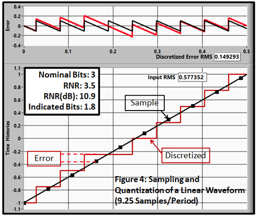
This shows the importance of realizing that the process is actually two steps:
- Sampling at equally spaced steps in time.
- Quantizing the signal at the points to the amplitude resolution (Range/2N).
So, the derivation only works properly for a straight-line waveform sampled at the correct time points.
If we change to a sine wave, we get Figure 5.
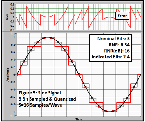
Figure 6 shows the result for a wiggly signal.
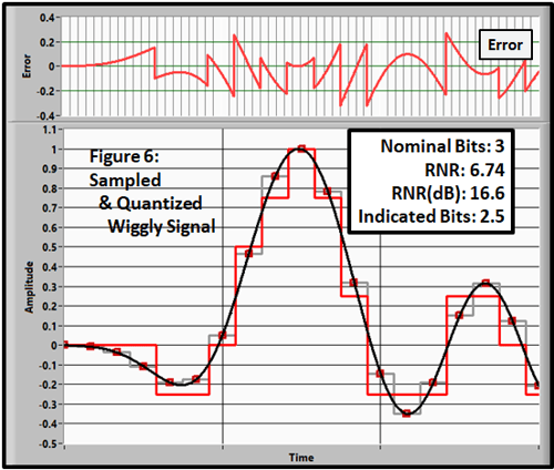
In all of these non-idealized cases, the Indicated Bits are significantly lower than the Nominal Bits. The errors are over-estimated.
Conclusion: According to this model, the quantizing range-to-noise ratio depends on the signal. It works for a straight-line signal that is synchronously sampled. The errors for other cases are significant.
But this model/concept is completely wrong.
The “Shannon View” of the Process
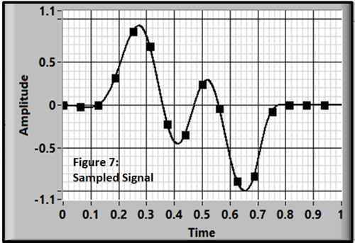
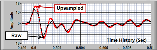
Let’s go back to basics. We are acquiring data at discrete points in time (Figure 7).
Those of you that have read my earlier blogs know that:
- if you believe in Shannon’s theorem (and we do, right?)
- and if we have a time history that is sampled fast enough (all significant frequency components are below the Nyquist frequency (S/2) satisfying Shannon’s Theorem).
we know everything about the signal. It is smooth and continuous...not made up of steps.
|
For example, in Blog 7, I discussed one of the methods that can be used to rebuild (upsample) the time history to any reasonable time-point spacing.
|
Analyzing the Signals Using the "Shannon View"
If we quantize the straight-line example using this strategy, we get Figure 8.
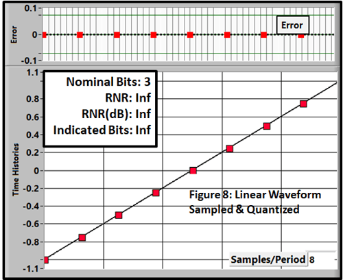
The quantized points fall exactly on the input data and the error is zero. The RNR and Indicated Bits are infinite! This is the case for all sample rates that are an integer multiple of 2N samples/period.
If we change the sample rate slightly, so the sampled points don’t fall directly on the line, we get Figure 9.
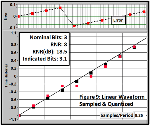
The resulting RNR and Indicated Bits are close to the value predicted by our basic equation.
Sampling and quantizing the data in Figure 6 produces the results in Figure 10.
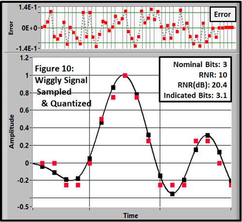
In this case, the Indicated Bits is a little high but much closer than the classical approach.
Ten experiments with similar waveforms produced results with an average of 2.77 with a max of 3.7 and a minimum of 2.7. With different time histories, you will obviously get different results.
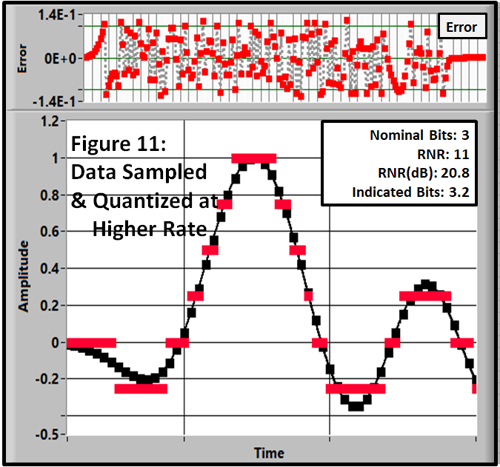
Increasing the sample rate has a small effect on the Indicated Bits (Figure 11).
Higher Resolution Analysis
Nobody really cares about 3-Bit Systems. They are just good to demonstrate basic ideas in a way we can easily see.
Figures 12 and 13 show a result of 12-bit quantization at 16 and 90 samples/sec.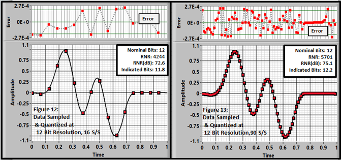
Again, the Indicated Bits is close but not exact.
Experiments with the full sample set produced a mean of 11.8 Indicated Bits with a maximum of 12.1 and a minimum of 11.4. Again, the basic relationship above produces a good approximation.
And the relationship holds pretty well for a random signal with higher frequency content (Figure 14).
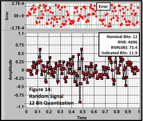
The “Shannon View” produces a good approximation of the effective bits for all of the waveforms analyzed.
The Strange Relationship: SNR(dB) (or RNR(dB) = 6.02 N + 1.76
So far, using the definition of RNR of:
RNR=RMS(Range)/RMS(Noise)
we have found that the RNR to be Eq.2.
RNR(dB) = 6.02 N
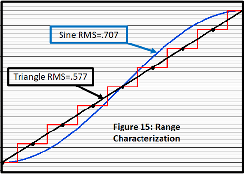
However, the standard RNR definition assumes a sinusoidal characteristic instead of a straight line (Figure 15). So the definition is
RNR=RMS(Sine(Range))/RMS(Noise) (7)
instead of Equation 1. Then
RNR=.707 x Range/(.5773 x Range/2N)
=1.22/2N (8)
Which leads to
RNR(dB) = 6.02 N + 1.76 (9)
Conclusion
Using the “Shannon' View” approach, the theoretical number of effective bits due to the sampling and quantizing process depends on the signal but is approximately
N=(RNR(dB)-1.76)/6.02
and hence:
RNR(dB)= 6.02 N + 1.76
which (remarkably, in my opinion) agrees with the fundamental result in References 1 and 2.
….except for the unique example of a properly sampled straight line where the equations produce an RNR and Indicated Bits of ∞. That case will probably never be encountered in practice.
In any case, more bits are good to a point. In an upcoming blog I will show that for many laboratory applications, 16 bits is an excellent match for the expected analog noise levels. More bits are wasted in those applications.
References
- Taking the Mystery out of the Infamous Formula, "SNR = 6.02N + 1.76dB," and Why You Should Care Walt Kester Analog Devices MT001
- Quantization Noise: An Expanded Derivation of the Equation, SNR = 6.02 N + 1.76 dB Ching Man, Analog Devices MT-229