
Vibration Signal Processing and Anomaly Detection Dashboard
Vibration signal processing is the analysis of sensor data from rotating machinery, using tools like FFT, PSD, and STFT, to detect mechanical faults before they cause failure. Pairing these techniques with machine learning anomaly detection, such as Isolation Forest and PCA, makes it possible to flag imbalance, misalignment, and bearing wear automatically. Typically, our posts are for educational purposes, but in this post we talk specifically about using enDAQ sensors and enDAQ sensor data to help with signal processing. In this guide, you'll learn how to explore enDAQ vibration data (.ide files) and use an interactive dashboard to visualize signals, run frequency analysis, and detect anomalies, helping you reduce downtime and move toward predictive maintenance.
Contents
-
- Histograms and Data Distribution
- Data Drift and Statistical Metric
-
Advanced Methods: Machine Learning for Anomaly Detectio
-
Final Thoughts: The Importance of High-Quality Vibration Data
Advanced Methods: Machine Learning for Anomaly Detection
As systems become more complex, traditional methods may not capture subtle or multidimensional patterns. Machine learning offers powerful alternatives (read the blog “Detecting Anomalies in Belt-Driven Systems with Machine Learning” here for deeper details on ML for anomaly detection).
Principal Component Analysis (PCA)
PCA reduces data dimensionality while preserving key variance. In vibration analysis:
- It captures dominant motion patterns
- Reconstructs signals
- Flags anomalies based on reconstruction error
Isolation Forest
Isolation Forest is an unsupervised algorithm designed to detect anomalies by isolating rare patterns in data. It works well for:
- High-dimensional signals
- Large datasets
- Unknown fault conditions
Other Advanced Models
Beyond PCA and Isolation Forest, more sophisticated approaches include:
- LSTM (Long Short-Term Memory) for time-series prediction
- Autoencoders (AE) for deep anomaly detection
- Hybrid physics-informed ML models
Dashboard Overview: Interactive Vibration Analysis
These methods enable predictive maintenance and intelligent diagnostics.
To bring all these methods together, the provided dashboard offers an intuitive interface for vibration analysis. In this section, uploading ide file and exploring different sections of the dashboard is explained. To do this, navigate to the dashboard link, click on the “Upload” box, and select your IDE file (a sample ide file is provided in download section at the end of this blog). For optimal performance, it is recommended to use a smaller IDE file to avoid time-consuming analysis during the machine learning–based anomaly detection process.
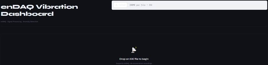
After uploading the IDE file, a sidebar will appear where the user can adjust the parameters. By moving the cursor over the “?”, a tooltip will display an explanation of each parameter. All sidebar parameters are described in detail in the section below.
Dashboard Link
Sidebar: Control Panel
The sidebar is the control center of the dashboard, allowing users to configure analysis parameters:
| Parameter Group | Dashboard View |
|---|---|
|
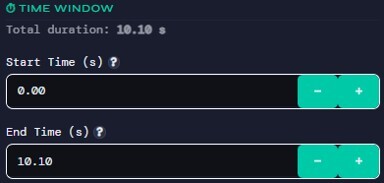
Time Window Selection
|
 |
|
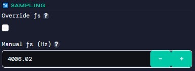
Sampling Settings
|
 |
|
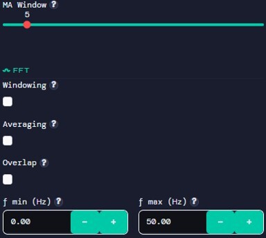
FFT Configuration
|
 |
|
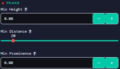
Peak Detection
|
 |
|
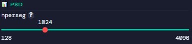
PSD Settings
|
 |
|
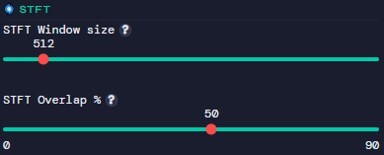
STFT Parameters
|
 |
|
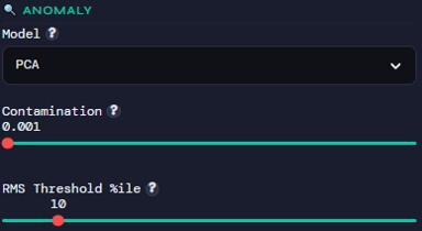
Anomaly Detection
|
 |
|
 |
Tabs: Organized Analysis Views
The dashboard is divided into multiple tabs, each focusing on a specific aspect:
- Time Series
- Raw acceleration signals (X, Y, Z axes)
- Immediate visualization of system behavior
- Statistics
- Histograms of vibration amplitude
- Key statistical metrics table
- FFT / PSD
- Frequency spectrum with peak detection
- Power spectral density plots
- Time–Frequency
- STFT spectrogram for dynamic analysis
- Anomaly Detection
- Machine learning-based anomaly identification
- Visualization of detected abnormal points
How to Use the Dashboard
- Upload an .ide file (enDAQ format)
- Adjust parameters in the sidebar
- Explore each tab for different insights
- Run anomaly detection to identify unusual behavior
Example Workflow
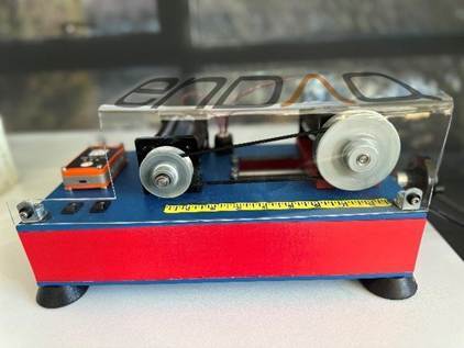
A sample dataset was collected by mounting an enDAQ sensor on a belt-driven machine, with the Z-axis oriented normal to the ground (Fig. 1). The data was recorded over a 15-second interval, during which five controlled impacts were applied to the machine frame using a pen to simulate anomalies. This dataset, provided as an IDE file, is used throughout the blog to demonstrate and walk through the features of the dashboard.
Once an .ide file is uploaded:
- The system automatically extracts acceleration data
- Sampling frequency is estimated
- Signals are preprocessed (e.g., detrending)
Step-by-Step Interpretation
- Time Series Tab
- Observe signal stability and periodicity
- Statistics Tab
- Check RMS and variance for abnormal increases
- FFT / PSD Tab
- Identify dominant frequencies and harmonics
- STFT Tab
- Detect time-varying frequency behavior
- Anomaly Tab
- Highlight segments flagged as abnormal
- Compare model outputs (PCA vs Isolation Forest)
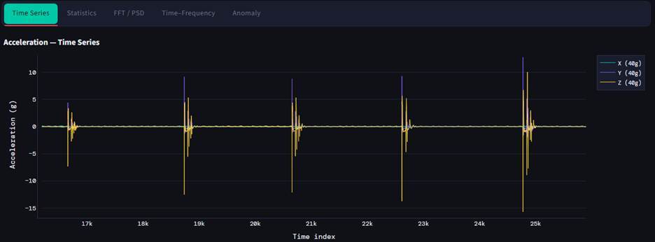
The time‑series plot clearly shows five high‑energy impact events across the X, Y, and Z acceleration channels, each producing sharp spikes that rise well above the baseline vibration level. Between impacts, the system remains stable with minimal variation, reflecting normal steady‑state behavior of the belt‑drive setup. The consistency of the spike shapes across axes indicates that each impact introduces a similar mechanical disturbance. Overall, the plot provides a clean visual separation between regular operation and externally induced shocks.
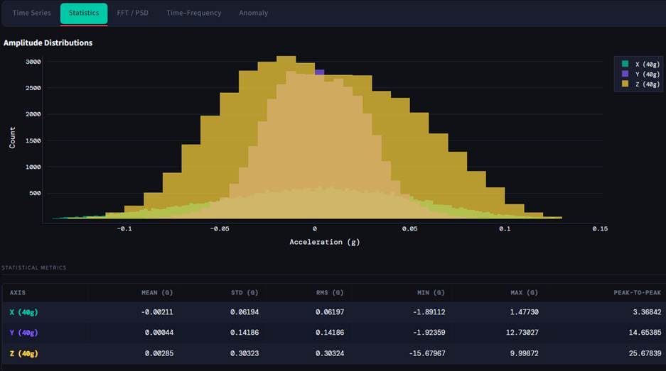
The amplitude distribution histogram shows that all three acceleration axes follow a roughly bell‑shaped pattern, with most vibration values concentrated near zero and gradually tapering toward the extremes. The Z‑axis displays noticeably wider spread and heavier tails, which is confirmed by its higher standard deviation and peak‑to‑peak value in the table. Meanwhile, the X and Y axes remain more tightly clustered, indicating more stable baseline motion in those directions. The statistical metrics reinforce these observations, highlighting how the Z‑axis captures the strongest variations and is most sensitive to impact‑driven disturbances in the system. Overall, the combined plot and table provide a clear overview of how vibration energy is distributed across the three axes during operation.
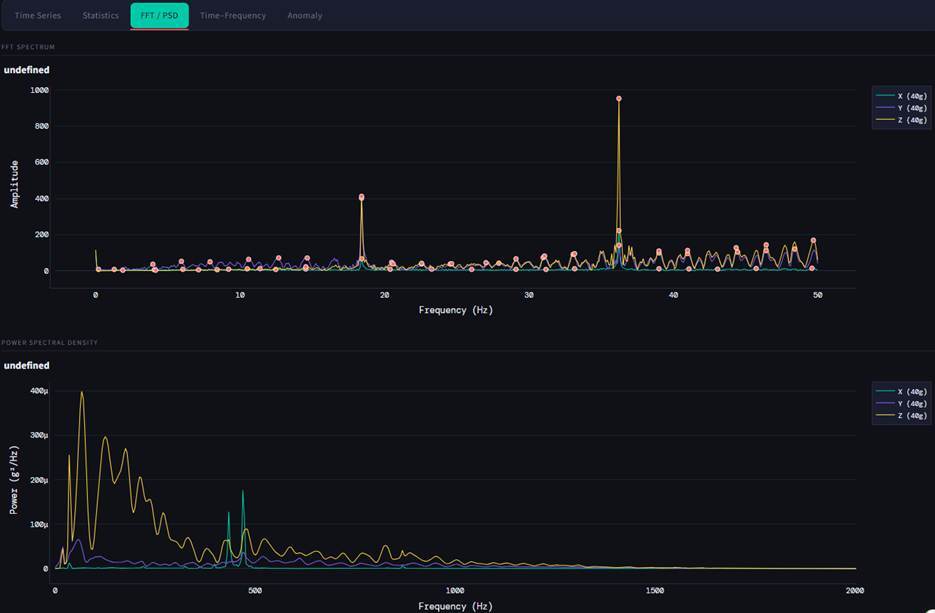
The FFT spectrum in the Z direction shows two clear dominant peaks, which can be attributed to the drive and driven pulleys of the belt system. The amplitude differences across the X, Y, and Z axes highlight directional sensitivity, with the Z-axis exhibiting the highest energy concentration due to its alignment normal to the machine frame. In the PSD plot, most of the signal energy is concentrated at lower frequencies, followed by a gradual decay, which is typical for vibration responses dominated by fundamental modes and their harmonics. The presence of these distinct peaks in both FFT and PSD indicates structured, repeatable behavior rather than random noise, while any additional broadband content may be associated with the induced impacts or other transient anomalies.
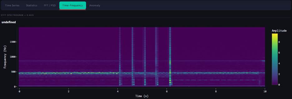
The spectrogram of the belt‑drive system shows a steady tonal band near the lower‑mid frequencies, representing the continuous rotational motion of the belt. Five distinct vertical bursts appear between roughly 4 and 7 seconds, each corresponding to an intentional impact made on the frame. These transients inject broadband energy momentarily, standing out clearly against the otherwise stable operating signature. Overall, the plot highlights how external mechanical shocks contrast sharply with the system’s normal, steady‑state vibration pattern.
PCA:
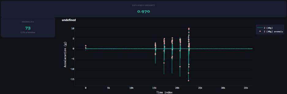
The PCA‑based anomaly detection highlights 73 anomalies in the Z‑direction, supported by a high explained variance of about 0.97, showing that the reduced components preserve most of the vibration behavior. The anomalies align closely with the five intentional impacts, forming tight clusters around these high‑energy events. This indicates that PCA is more selective, emphasizing broader structural deviations rather than small, isolated spikes. As a result, it offers a more conservative but stable view of abnormal behavior, making it well‑suited for detecting consistent pattern changes caused by repeated impacts.
Isolation Forest:
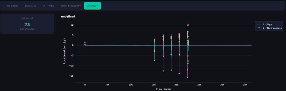
The anomaly plot highlights how the Isolation Forest model responds to the five intentional impacts introduced into the belt‑drive system. While it successfully identifies the main shock events, it also flags numerous smaller fluctuations around them, resulting in a much higher anomaly count. This reflects the method’s sensitivity to short, abrupt deviations in vibration behavior, making it well‑suited for early fault detection. However, the increased responsiveness also means that more benign variations may be labeled as anomalies.
Final Thoughts: The Importance of High-Quality Vibration Data
All the techniques discussed, whether statistical, spectral, or machine learning, depend heavily on one critical factor:
“Data Quality”
Poor-quality data leads to:
- Misleading frequency content
- False anomalies
- Missed fault signatures
High-quality vibration data must have:
- High sampling rates to capture fast dynamics
- Low noise levels
- Accurate calibration
- Reliable synchronization
High quality sensors play a crucial role. They are designed to capture high-resolution, high-fidelity vibration data, enabling precise analysis across time and frequency domains.
Such high-quality data is essential not only for traditional condition monitoring but also for emerging applications like:
- Anomaly detection systems
- Predictive maintenance pipelines
- Agentic AI systems interacting with physical environments
- Physical AI and digital twins
In modern engineering workflows, data is the foundation, and better data leads directly to better decisions.