Shock Analysis: Response Spectrum (SRS), Pseudo Velocity & Severity

Shock analysis doesn't need to be so complicated. How would an engineer compare the shock severity of these 5 different events?

1. Motorcycle crash with a car
2. Human hitting a punching bag
3. Earthquake
4. MIL-S-901D (military standard for shock testing of equipment on Navy ships)
5. Recoil of gun stock during firing

Many people jump to comparing the peak acceleration value which we'll prove is not only inadequate but often misleading. But there is a way to summarize a shock event into a single metric that measures severity: pseudo velocity!

In this post I'll try to provide the right mix of theory and practical information, with examples, so that you can hopefully take your shock analysis to the next level!

You may be more interested to jump to the comparison of the real data (which can be freely downloaded). It is important to understand the theory first, but I'll use plots to make my point instead of only equations and text. And all these plots are generated with a truly free software tool.

In this post we'll cover the following:

1. Shock Analysis Basics
1. Shock Analysis in the Time Domain
2. What is a Shock Response Spectrum (SRS)?
3. What is Pseudo Velocity?
4. Filtering vs Integration vs Pseudo Velocity SRS
5. What is a Severe Shock?
2. Comparisons
1. Generated Half-Sine Pulses with Varying Amplitude & Width
2. Generated Pulses with A Lot of Zero Data
3. Impact of Sample Rate
4. Impact of Different Damping
5. Comparison of Real Application Examples
3. How to Act Upon Your Analysis
4. Tools to Calculate Your Own Pseudo Velocity SRS
5. Conclusion & Additional Resources

Let's go through how to analyze a shock event! You'll be doing your shock analysis in the real world so we'll look at real world examples, and analyze data captured from an actual accelerometer. But first, let's start with the basics.

Shock Analysis Basics

Shock Analysis in the Time Domain

When looking at shock data you'll likely see it in the time domain: a plot of acceleration amplitude (normally in 'g' which is 9.81 m/s²) vs time (normally in seconds). The plot below compares 5 different standard "half-sine" shock pulses of different amplitudes (1, 10, 25, 50g, & 100g) and different pulse widths (500, 50, 20, 10, & 5 milliseconds or ms).

The most obvious metric that jumps out at you is the maximum amplitude of the event. But this information alone does not provide a full description of the shock event. The pulse width is also needed or, ideally, a shock response spectrum (SRS) is used to characterize the event. In general, analyzing shock data in the time domain is insufficient, like vibration, because most real world shock pulses are made up of many frequencies.

Let's look at some raw acceleration data taken when a Kawasaki motorcycle (with an enDAQ sensor mounted in the CG) is impacted by a car (remember all data shown in this post is available to download!). There is a peak acceleration at 120g, but there is clearly a lower amplitude (60g) and much longer duration (60 ms) pulse that is also present and likely much more damaging. Clearly, relying solely on one peak amplitude and pulse width isn't enough to characterize a real world shock event!

So what is used to characterize a shock event? When doing shock testing you are generally worried about potential damage and therefore energy becomes the concern. We know kinetic energy is equal to 1/2 * mass * velocity². Note how acceleration isn't in there! This velocity is the area under the curve of the acceleration data. 

But we don't want to solely look at that area and singular metric, rather we will get a much richer description of the event if we understand the energy at the system's modal frequencies. As we'll discuss next, the pseudo velocity shock spectrum (PVSS) is a simple and informative way to do this energy-at-frequency analysis!

What is a Shock Response Spectrum?

Before we can discuss pseudo velocity, we need to understand what a shock response spectrum, or SRS, is. It calculates and defines how a single degree-of-freedom system with different hypothetical natural frequencies would respond to the shock. To illustrate how this is helpful, let's take that 50g, 10ms pulse and calculate how a system with a 30 Hz, 85 Hz, and 250 Hz natural frequency responds to that input.

The hypothetical system with a 30 Hz natural frequency experiences the same overall peak acceleration level, but its response looks very different to a 250 Hz system which tracks the pulse. And the 85 Hz system is actually magnifying the input pulse and experiencing a higher acceleration level to that pulse. A shock response spectrum loops through many hypothetical natural frequencies of a single degree of freedom system and determines the maximum acceleration they would experience as shown.

Looking at this shock response spectrum an analyst can conclude that systems with natural frequencies below 30 Hz are attenuating the input (isolating) while frequencies above 250 Hz are "hard mounted" and tracking the input. But between those frequencies, a system is actually magnifying the input! So the SRS is helping identify how your system (and components within the system) would respond to a shock event.

One of the other primary benefits of the SRS is that by being in the frequency domain, converting to velocity and displacement is quite simple. And as we'll find next, velocity is more indicative of the damage potential of a shock event than acceleration levels.

What is Pseudo Velocity?

Pseudo velocity is equal to the relative displacement SRS (difference between input and response) multiplied by each corresponding w_n (2 * pi * natural frequency). To show how the pseudo velocity is calculated, let's start by revisiting our example and the relative displacement response to the 50g 10ms pulse.

Now we'll do the same shock response spectrum approach and calculate how a series of different natural frequencies would respond to that input in the relative displacement SRS. Notice how the peak response relative displacement (absolute value) in the time series data above, corresponds to the displacement shock response spectrum values below.

Now let's get a little crazy and pull in the pseudo velocity shock spectrum (PVSS). This plot can initially make your head hurt, but when you get used to it you can fully realize its value. This is called a tripartite or four coordinate plot because it is not only providing the pseudo velocity relationship but also includes the displacement (diagonal from bottom left to upper right) and acceleration (diagonal from upper left to bottom right). See how that 250 Hz data point called out that is on the 0.008 inch diagonal and 50g diagonal (highlighted in red) which matches what we saw in the relative displacement and acceleration shock response spectra. The two lines are for negative and positive peaks in that oscillating response, but for the rest of the article we'll focus on the maximum between the two.

Now let's do that same progression with some more interesting data of that motorcycle crash! First here is the acceleration response in the time domain of three different natural frequencies: 10 Hz, 100 Hz, and 1 kHz. And we've called out the peak acceleration each one of those frequencies experiences.

Now in the acceleration response spectrum those three natural frequencies, as well as the full range between, is plotted. 

Now we do the same with the relative displacement between an input pulse and the response of a system (important to help with isolator design). The 1000 Hz system has a very small "wiggle" while the 10 Hz system has a relative change of almost 7 inches!

Now here is the relative displacement shock response spectrum.

Now we bring it all back together and show the pseudo velocity shock response which gives us the other metrics (acceleration and relative displacement) in that one plot! For a nice high resolution image of below to zoom in, click here. I do want to again remind you though that the acceleration response is being approximated (very well I may add) by using the relative displacement multiplied by w_n for pseudo velocity, and then again for the acceleration. Different damping will effect this approximation.

For a more thorough technical explanation on what pseudo velocity is and why it is so important, please read Pseudo Velocity Shock Spectrum Rules For Analysis Of Mechanical Shock by Howard Gaberson, the original champion of pseudo velocity. But let's continue by demonstrating the power of it!

Filtering vs Integration vs Pseudo Velocity SRS

Let's go back to our cool shock data of when a motorcycle was impacted by a car. That had a lot going on, so let's start by seeing what happens when we apply low pass Butterworth filters at 160, 80, 40 and 20 Hz.

It's hard to compare the event with the raw data because it is so "messy" so let's remove it for an easier comparison... now this data is starting to be much more digestible and relevant.

But wait! You'll see the maximum amplitude of the plot is less than 70g, surely the high frequency data we filtered away was important wasn't it?! No, not from a damage perspective.

Let's straight integrate the raw and filtered acceleration data to calculate the velocity change from this significant impact. Notice how the 160 Hz and 80 Hz filtered data's velocity change is identical to the unfiltered. The 40 Hz filtered data even is very close while the 20 Hz is clearly too aggressively filtered. In a way, this is indicating that integration itself effectively "cleaned" the data, notice how clean that previously noisy acceleration data is once integrated!

Now let's look at the pseudo velocity shock response spectrum for all of these different applied filters.

I want you to notice from this pseudo velocity SRS comparison that the plateau/maximum pseudo velocity corresponds closely to the velocity change from the impact itself. So what have we learned?

1. Digital low pass filtering is helpful to "clean" a shock event while still not influencing the total energy or damage potential
2. The maximum acceleration amplitude doesn't tell you much of anything
3. The velocity change from a shock event can in effect "clean" the data because the high frequency components have less of an impact
4. The pseudo velocity SRS can do all of the above and more in one plot!

Let's look at the four coordinate pseudo velocity shock spectrum (PVSS) of this event below.

1. The plateau at the ~630 in/s matches the velocity change from integration (and as we'll find out in the next section - this is a very severe event that will probably cause damage, as one would expect from a motorcycle/car crash). We'll also show that with less damping, this approximation becomes even more accurate later.
2. Acceleration peaks (shown on the downward diagonal from upper left to lower right) at slightly over 100g at the higher frequencies, again matching what we saw in the raw time series data
3. That plateau ends around 6 Hz at an acceleration diagonal of 50g which corresponds nicely with the peak acceleration and pulse width (80ms) of the 40 Hz filtered data - in effect, the pseudo velocity did some filtering for us

And it does all this in one plot! Now let's explain why we keep saying that pseudo velocity correlates more to damage than acceleration and therefore is more important.

What is a Severe Shock?

As we mentioned when looking at the time domain data, the energy in a shock event is the area under the curve. Stress is proportional to modal velocity, not g's or acceleration. From equation 16 in Gaberson's paper:

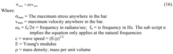
We know stress limits for materials and therefore can calculate the maximum velocity for these materials. The following provided table is from Tom Irvine's Introduction to Shock & Vibration Response Spectra, Chapter 19 on Pseudo Velocity. As another reference, Tom also shared a presentation on pseudo velocity severity on his website in June 2020.

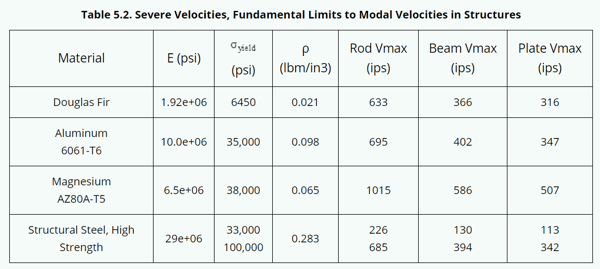
Another paper by Gaberson on Shock Severity provides the following table.

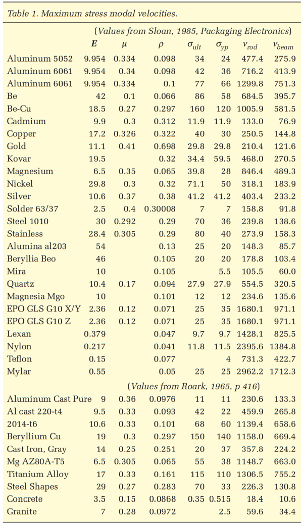
Notice how there is a velocity value for each material at which it starts yielding and some of these approach 100 inches per second (ips) in the case of steel and even fall below that in materials like solder (electrical systems) and concrete is all the way down at 10 ips.

In addition to Gaberson and others, we've seen military standards specify shock severity in terms of velocity. MIL-STD-810E and SMC-TR-06-11 stated that a shock is considered "severe" if one of its components exceeds the threshold of 0.8 (G/Hz) * Natural Frequency (Hz). This is effectively a velocity criteria that works out to 50 inches per second. MIL-STD-810E also states that based on unpublished observations that military quality equipment does not tend to exhibit shock failures below a shock response spectrum velocity of 100 inches per second (which makes that earlier equation a 6 dB margin of conservatism).

So let's summarize these values into a simple rule-of-thumb risk gauge for categorizing shock severity. Note these are guidelines and there will be some exceptions.

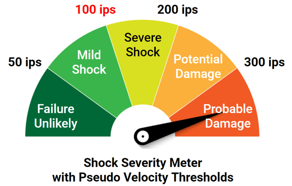
Generally, the 100 inch per second (ips) threshold for pseudo velocity is used in industry as that threshold for defining a "severe" shock.

Comparisons of Different Shock Events

Enough theory and math, let's compare some example shocks!

Generated Half-Sine Pulses with Varying Amplitude & Width

Let's revisit that comparison of the 5 different standard "half-sine" shock pulses of different amplitudes (1, 10, 25, 50g, & 100g) and different pulse widths (500, 50, 20, 10, & 5 milliseconds or ms).

You can just barely see the 1g shock yet it lasts a long time! You may be quick to assume that the 100g event is the most severe because it has the highest amplitude... but you would be wrong. They are all equally as severe. Here's the pseudo velocity SRS.

The exception to the statement that they are all equally severe is that if we know our system has no components with low natural frequencies, then the pulses with high pseudo velocities at higher frequencies are more worrisome. 

I hope this highlights that amplitude is really insignificant in characterizing a shock event, the duration and other frequency components to the event are more major drivers of damage potential. Now let's see the impact of how often a shock happens in a 60 second period. Can the SRS capture that and highlight the increased damage potential?

Comparison of Pulses with A Lot of Zero Data

One of the major benefits of the SRS is that it calculates the maximum response per natural frequency. It isn't a pure frequency spectrum which can get impacted by the time length and something we talk about with vibration analysis. To highlight this, let's compare a PSD of that 50g, 10 ms pulse with only 0.19 second of "dead time" compared to one that is 60 seconds long. The vast majority of the time is zeros as that shock event is short. If we calculate the PSD we would significantly mute that event.

But when we compare the pseudo velocity (holds true for acceleration and displacement) the response is identical! This lets us compare different shock pulses with varying time lengths or "weak vibration/shock" around the main pulse in a single simple plot.

Impact of Sample Rate

The motorcycle data was sampled at 10 kHz but as we saw in the filtering section, the bulk of the data was at frequencies below 200 Hz so they could have arguably sampled at 1 kHz. Although it is always easier to reduce data than add so err on the side of sampling too high!

But let's look at another real world example that was sampled appropriately at 20 kHz, the gun stock. This was again using our enDAQ sensors which had a very robust 4 kHz low-pass filter to prevent aliasing. We can apply a low pass filter to this data and decimate the signal to simulate what an accelerometer would have measured if it wasn't sampling fast enough. But this assumes your system is using a good low-pass filter! See the different measurements in the time domain with sampling at only 2 kHz (and a 400 Hz filter) and 1 kHz (with a 200 Hz filter).

Looking at this data one may suggest that the 1 kHz sampled data is clearly undersampled. But how would an engineer know that? They may think that half-sine pulse it's tracking is the entirety of the event with an 80g peak and 6 ms pulse width, when the real event was actually about a 420g peak with a 1.5 ms pulse width. The answer... pseudo velocity! Let's compare the PVSS between the three signals.

1. The pseudo velocity shock spectrum of the full 20 kHz sampled data tracks exactly with the 2 kHz sampled data and very closely with the 1 kHz sampled data - which means pseudo velocity effectively eliminated the effect of sample rate on how we analyze a shock!
2. But also notice how clearly the PVSS ends somewhat abruptly after reaching that peak of about 100 in/s. Because I'm not seeing the PVSS decline fully (ideally a factor of 10, but at least a factor of 2) from the peak, I know that I undersampled that event and there may be information there that was missed. The PVSS can identify if the shock event had been undersampled! Although thankfully even the undersampled data still all equally characterized the severity of the event. 

The Impact of Damping

Throughout this article I have been using a damping coefficient of 5% or a Q of 10. How does damping effect the results of the PVSS? Well pseudo velocity is measuring a response to an input, so the more damping you have the lower that response will be as you can see below. 

Comparison of Real Application Examples

I've given a lot of focus to the half-sine pulses, but I'd guess that crash test data is the most interesting! Now that we have worked through a lot of theory, let's compare some real-world events that you can relate to. Remember all data shown in this post is available to download.

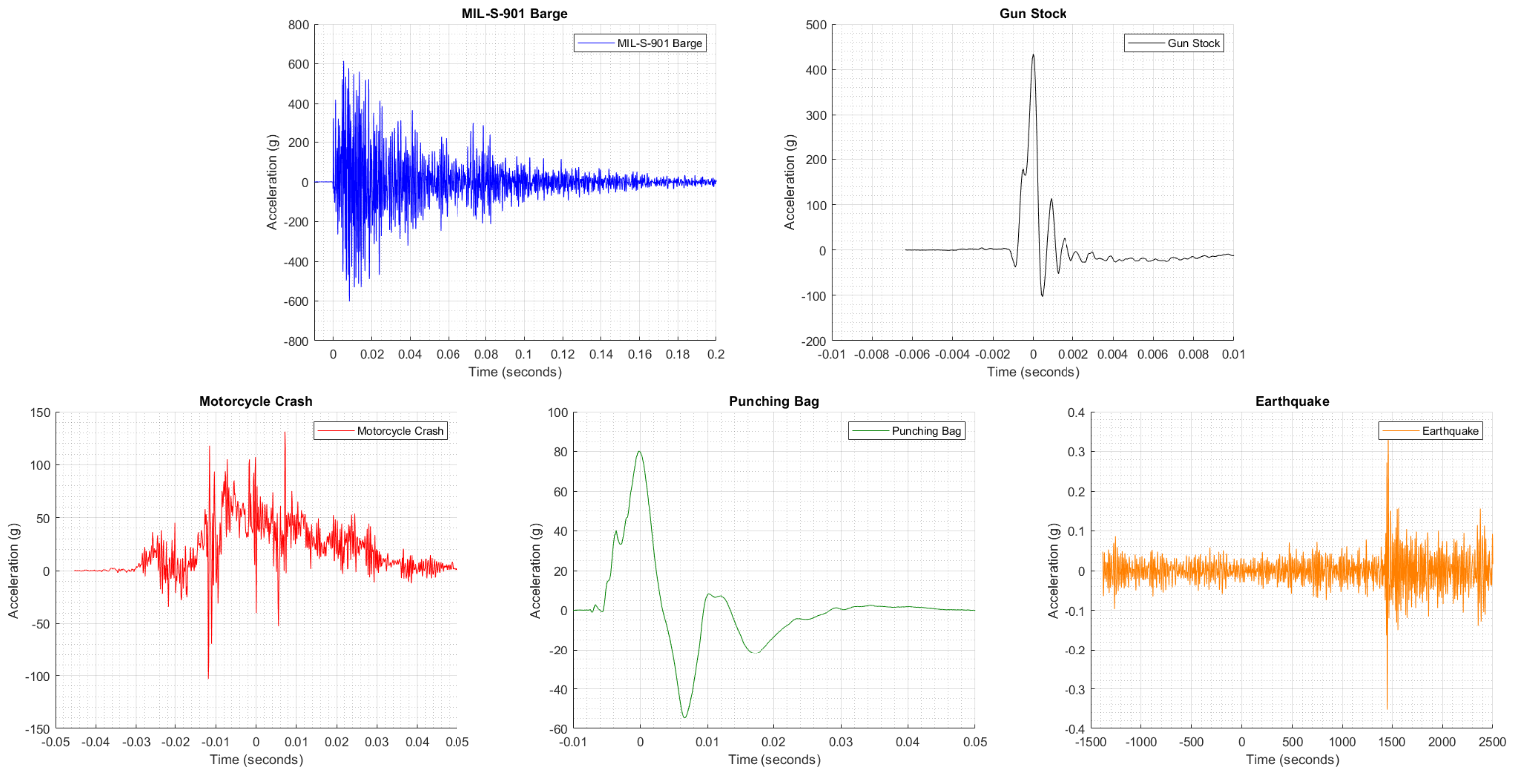
• MIL-S-901 Barge Shock: This is a test standard that defines a very "severe" shock event such as a torpedo impact to a ship. But not only military applications utilize this intense test standard, Amazon and AWS recently used it to test their portable data centers. It is achieved at a few test locations around the country (Mide has used HiTest in VA for our sealing systems on destroyers, where this raw data came from).
• Gun Stock: This is from a Greyboe who we did some testing with to prove the superior damping on their composite gun stocks. But even with that better quality stock, the shock of the recoil when the gun is fired is intense.
• Motorcycle Crash: This data is cool and part of a study Momentum Engineering Corp. published on motorcycle-vehicle impacts and the resulting change in velocity. It is a real motorcycle (Kawasaki) with a dummy on it, impacting a vehicle (Malibu) with an enDAQ sensor mounted to the center of gravity on the motorcycle (no big deal, it can survive that impact!).
• Punching Bag: This is also data taken with an enDAQ sensor mounted to a punching bag when someone punches it as hard as they can
• Earthquake: This is the only dataset not from an enDAQ sensor, but courtesy of Tom Irvine from a 6.8 magnitude earthquake measured in the Solomon Islands in 2004. Here's a report of the source of this data and more information on earthquakes.

Let's look at the comparison of the acceleration data from these events shown in the time domain. You can see that this looks ridiculous. It is not an effective way to compare shock events of varying amplitudes and durations!

Here are the 5 events individually plotted and compared:

So let's get to the main event and calculate and compare the pseudo velocity comparison of these events, which you can see in a simple and clean single plot.

All of these events are "severe" shocks or greater, surpassing the 100 ips pseudo velocity threshold. But believe it or not, the earthquake is the most severe logging a maximum pseudo velocity of about 1,000 in/s! Yet, the maximum acceleration amplitude in the time domain was 0.3g. Clearly, "max g" or peak acceleration is a misleading way to characterize a shock event. And it shouldn't be all that surprising when we remind ourselves that earthquakes are capable of toppling buildings.

If there is one takeaway I want you to have from this article, it's that acceleration peak amplitude is a completely inadequate and misleading metric to use in characterizing a shock event. I also hope you can recognize above that the pseudo velocity SRS is a nice way to compare multiple events which are otherwise difficult to compare in the time domain.

How to Act Upon Your Analysis

If all you were interested in is characterizing if your shock is "severe," then you would be done at this stage! But often the engineer needs to take one more step and protect the system if it is needed. You have three options:

1. Do nothing because the pseudo velocity is below 100 in/s and not severe
2. Isolate your system from the shock with a low frequency isolator
3. Hard mount by stiffening the coupling 

If you go the route of isolating your system you'll want to work with a company like Hutchinson Inc. (formerly Barry Controls) that specializes in solving shock and vibration problems for the US military. They, or any other isolator company, will turn to the pseudo velocity SRS to help guide their design and recommendations on how to develop an isolator. This process deserves a dedicated full feature blog to explain, but the shock response spectrum, specifically the pseudo velocity 4 coordinate plot, comes in handy. Below I've included the plot for the gun stock.

The peak pseudo velocity was just over 100 ips so let's consider that we decide to use a 3 Hz isolator to bring it down to about 18 ips. But I can see here that this requires a near 1 inch of relative displacement (see the bottom left to upper right diagonals) which would drive the size and design of my isolator. And if I go the other way and decide to hard mount it with a 1,800 Hz coupling, it too will bring down the maximum pseudo velocity to a similar 22 ips. But it requires the system enduring acceleration levels at 600g which is amplifying that ~400g input. There are always trade-offs in engineering!

Tools to Calculate Your Own Pseudo Velocity SRS

Capture Shock Data

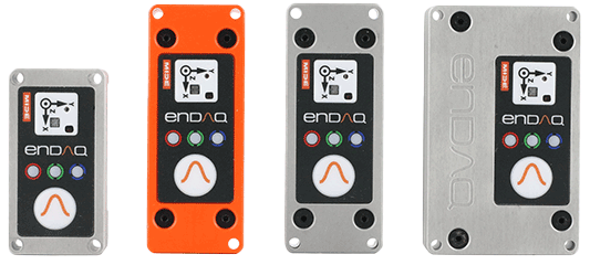
You'll need some acceleration time series data to use to calculate your own SRS.  In order to get that data you can use some traditional accelerometers (see our article on accelerometer types and where to buy them) or you could consider a shock data logger (see our article on the top 11).  Pictured here are our portable and multifunctional enDAQ sensors that were designed to be brought out into the field to quantify shock & vibration environments. Our units include an option to use a piezoresistive accelerometer which is ideal for shock testing, and an amplitude range up to 2,000g.

Calculate the Shock Response Spectrum with Free Software

All of the plots in this article were generated using our VibrationData Toolbox. You can download this software directly from our website. We also have a dedicated VibrationData Toolbox section in our Help Center with user guides to help you use this software to its full potential. Pictured here is the dialog for calculating the SRS off time series shock data where it also enables you to set the damping coefficient and other information.

If you'd prefer to calculate shock responses spectrums more directly with Python code, check out our post Top 12 Vibration Metrics to Monitor & How to Calculate Them which provides the source code to do it yourself!

Conclusion & Additional Resources

If there can be two things to take away from this post:

1. Characterizing a shock analysis based on the peak acceleration value is effectively useless and misleading
2. Pseudo velocity is a much more effective metric to characterize a shock event, especially with the full shock response spectrum

Expanding upon why pseudo velocity is the best!  There are a few advantages:

• Proportional to dynamic stress which in effect measures severity
• Maximum pseudo velocity is the impact velocity or velocity change that took place during the shock (which is why there is often a plateau)
• Easy to calculate and approximates the relative velocity which isn't easy to calculate
• More condensed view compared to acceleration SRS or relative displacement SRS
• Can infer the acceleration SRS and displacement SRS from the one plot of pseudo velocity shock spectrum (PVSS)

But don't just take me at my word, download the data used in this post or go measure your own data and do your own analysis!

Please don’t hesitate to leave a comment or contact us directly with any questions you may have on this topic or others. We are here to help you with all your testing needs!

Related Posts:

• Top 12 Vibration Metrics to Monitor & How to Calculate Them
• Accelerometers: Taking the Guesswork Out of Accelerometer Selection
• Why the Power Spectral Density (PSD) Is the Gold Standard of Vibration Analysis

For more on this topic, visit our dedicated Shock & Impact Sensors and Loggers resource page. There you’ll find more blog posts, case studies, webinars, software, and products focused on your shock testing and analysis needs.