The power spectral density (PSD) function is an excellent tool for analyzing vibration data such as acceleration, velocity, or displacement data because its output is independent of time duration (see our blog that explains more about this). But the units are g2/Hz which can be a little confusing, engineers are expecting to see the units as g which would mimic the output of a typical Fast Fourier transform (FFT)!
What if we could leverage the benefit of the PSD's calculation technique which involves averaging overlapping segments, but scale it so that the output has the expected units of g? What if there was an FFT function that gave an output you expected but gave you control over defining the frequency resolution? At enDAQ in our open-source Python library, we did just that! This blog will explain this calculation methodology and introduce the function you can use on your own data!
I will make the method available to you with our open-source software and show you examples of how it works using both some waveforms I have created and some vibration data from a medical instrument. Some of the plots will be interactive, so have fun zooming around in them! I will discuss the following topics:
In this blog, I will present:
- Video and Demonstration in Python
- Creation of a test signal
- Using the Aggregate FFT function
- How time interval and bin width affect the Aggregate FFT
- How the Aggregate FFT function works
- A real-world example
- Conclusion
Video and Demonstration in Python
Follow along with all the calculations in the video below and/or in this Google Colab that contains all the source code and interactive plots!
Creation of a Test Signal
First, let's generate three signals to simulate vibration data from a hypothetical device. One is random noise in the frequency range of 10 to 50 Hz. The two other signals are pure sinewaves with amplitudes of 1 g, one at 30 Hz and the second one at 80.25 Hz. The time domain composite signal over a 10 s interval is shown in Figure 1.
Figure 1. Time domain plot of the generated signals
Inspection of the waveform does not give you any real useful information other than an indication of the magnitude of the acceleration of the vibration data. We need to determine the frequencies where the vibration is dominant.
Using the Aggregate FFT Function
Before we explain exactly how the FFT calculation is performed, let's show you the output of our function: endaq.calc.fft.aggregate_fft(). This function allows you explicitly define the frequency resolution (this controls the length of the overlapping segments we'll discuss next), in this example, we set it to 1 Hz.
Figure 2 below is provided as a still image and an interactive plot as well so you can isolate certain signals by clicking in the legend. The magnitude of the 30 Hz sine wave is displayed as 1 g which is what would be expected. The plot of the 80.25 Hz sinewave shows a magnitude of around 0.9 g and not 1 g. This is due to the fact that the frequency, 80.25 Hz, does not align exactly with the center of a bin. The amplitude of the signal has leaked into adjacent bins so its peak at 80 Hz is a little lower than its total amplitude. Despite the minor difference in amplitude, the signal represents high vibration at 80.25 Hz. Then if you look at the random noise spectrum, you'll notice the amplitudes are relatively constant across this range as we'd expect.

How Time Interval and Bin Width Affect the Aggregate FFT
Now let me show you the Fourier transform data as a function of different time intervals and different bin widths. See Figure 9. Each row of plots represents a different bin width. The plots on the top row have a bin width of 0.5 Hz. The middle row plots were computed with a bin width of 1 Hz, and the lowest row used a 2 Hz bin width. The different color waveforms represent Fourier transforms of different time segments of the time domain data. Time segments include two seconds, three seconds, eight seconds, nine seconds, and 10 seconds.
The different time segments do not have an appreciable effect on the Fourier transform results. You can see that from the overlap in the plots of the sinewaves in the second column. You do see the amplitude of the 80.25 Hz increase to 1 g as the bin width widens and more of the frequency component is consolidated in a single bin. The wave shape also narrows similar to the 30 Hz sinewave which is centered in its bin.
Using the aggregate or averaged Fourier transform of the multiple time segments, you can see that the single frequency signals are properly identified independent of bin width. However, the wideband data represented by the 10 – 50 Hz noise does show an increase in amplitude and a smoothing of the magnitude of the Fourier transform as the bin width widens to include more spectral content per bin.
That results from the spectrum not being a computed power spectral density. The important point is if you are going to use an averaged Fourier transform for comparison between data sets, you need to make sure that all the data sets computing the Fourier transform using identical bin widths.

Figure 9. Plots of the Aggregate FFT with varying time segments and three different bin widths
How the Aggregate FFT Function Works
Let me tell you how the Aggregate FFT function works. First, you input the parameters required by the function:
- Input overlapping segmented time domain data
- Define the bin width
Figure 10 shows the segments of the time domain data entered into the Aggregate FTT function.
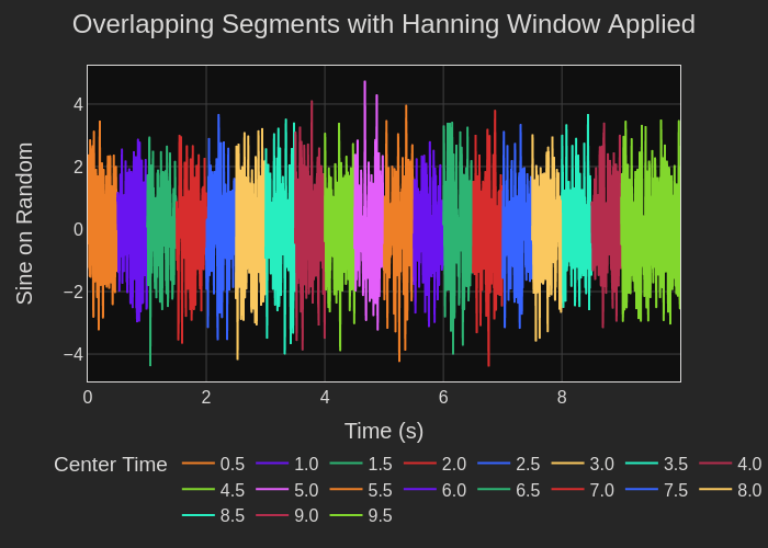
Figure 10. Plot of time domain data. Each color represents a different time segment.
The Aggregate FFT function does the following:
- Applies a boxcar filter, a square box filter, to create the individual data segments. Unlike with a power spectral density function, a Hanning window is not used preventing distortion of the time domain data.
- Computes a Fast Fourier Transform on each time segment (Figure 11)
- Squares and normalizes the Fourier transforms to the bin width
- Averages all squared, normalized Fourier transforms
- Multiplies by the bin width
↑↓ Converts from a PSD calculation to a processed Fourier transform result - Computes the square root
- Plots the result (Figure 12).
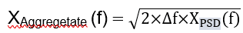 where Xpsd = the power spectral density, Δf = bin width, units are g.
Figure 5 shows plots of individual Fourier transforms for each time domain segment. The final result is the grey line in Figure 6 which shows the resulting averaged and processed composite Fourier transform of the data.

Figure 5. Individual Fourier transforms of each time segment

Figure 6. Plot of the output of the Aggregate FFT waveform, the grey waveshape, overlaying the individual FFTs
A Real-World Example
Let’s analyze some real-world data. Figure 7 shows 0. 1 s of acceleration data on all three axes from a surgical instrument. Seven peaks in 0.1 s suggest that the aggregate FFT should show a resonance peak at approximately 70 Hz. That is about all that the time domain data tells us.

Figure 7. Time domain plot of 0.1 s of vibration acceleration data from a surgical instrument. The x-axis, y-axis, and z-axis plots are overlayed on each other.
Using the Aggregate FFT function and specifying a 1 Hz bin width yields the results displayed over a 2500 Hz bandwidth shown in Figure 8. The plot shows a low frequency peak and a number of lower magnitude frequency components. If we zoom into the lower frequencies (it's an interactive plot!) we see the expected 73 Hz acceleration peak, and it has a magnitude of 1.15 g. Designers have the data they need to help them identify the source of the vibration and investigate ways to minimize the vibration at 73 Hz.

Figure 8. Frequency domain plots using the Aggregate FFT function. The plot is over a 2500 Hz bandwidth. Zoom in on the interactive plot to see the peak at 73 Hz.
Conclusion: Multiple Tools for Vibration Analysis
Now you have two tools for analyzing the frequency domain of a vibration signal, or really any signal! One is power spectral density analysis (see my blog on calculating a PSD) and now you have this modified PSD / FFT!
In this blog, I introduced the second tool, our Aggregate FFT function, to enable you to perform frequency domain analysis while maintaining the units you used to acquire your vibration data. You may find the Aggregate FFT function more intuitive to work with.
We have more information for you on using the enDAQ open source Python library for vibration analysis in the frequency domain. Subscribe to our library of videos on the subject. Feel free to take advantage of our open source Python library.