Real-world vibration data typically consists of a broad range of different frequencies that aren't obvious in the time domain. So engineers turn to the power spectral density (PSD) to represent a signal in the frequency domain which has the benefits over simpler Fourier transforms (FFT) because the results are independent of time duration, sample rate, or frequency bin width.
But to understand why power spectral densities are so effective, we first need to understand how to calculate a PSD! In this blog I'll show you how to calculate this using enDAQ's open-source Python library. But even if you don't plan to use Python, you'll still learn in this blog what goes into the underlying calculation of a PSD and how to use it to analyze your vibration data. We'll look at some artificially generated data, then real-world vibration data. The plots we'll include will be interactive too!
In this blog, I will present:
- Video and Demonstration in Python
- What is the Power Spectral Density Function?
- Using a PSD analysis of three artificial signals
- Demonstrating the nuts and bolts of the PSD Calculation
- An analysis of real-world vibration data
- Conclusion
Video and Demonstration in Python
Follow along with all the calculations in the video below and/or in this Google Colab that contains all the source code and interactive plots!

What is the Power Spectral Density (PSD) Function?
Vibration data as a function of time, time-domain data, can give information about the relative intensity of vibration, but time-domain data does not provide any information on the frequency or frequencies where the energy is concentrated. For frequency domain information, we need the power spectral density, PSD, which describes the distribution of the power of the time series data into frequency components.
The mathematical definition of the power spectral density function, XPSD(f), uses the discrete Fourier transform, X(f), of the time domain data, x(t), and is defined as:

For vibration analysis, the PSD represents acceleration, and the units of the PSD are g2/Hz in which g denotes the g-force. The factor, ½, converts the computation to a rms value. The Δf term is the inverse of the measurement time and equals 1/T.
The plot of the PSD function shows the frequencies where the vibration energy is concentrated. For more of a technical discussion on a PSD function, visit our learn article with a handbook download available.
Demonstration with three signals
Let's start by generating some data! Figure 1 shows the time-domain display of three signals. One signal is white noise in the frequency band between 10 and 50 Hz. Added to the noise are two sine tones, one is a 30 Hz sine wave and the second is a sine wave with a frequency of 80.25 Hz. The time-domain display does not provide much useful information other than the peak which is about the same for all! Remember, go ahead and zoom around in the plot!
Let’s see what we can learn from the frequency domain. This is where the PSD can help. Using our open-source library obtaining a PSD is quite simple with the function endaq.calc.psd.welch():
- Provide as input the time domain data indexed by time
- Select a frequency bin width
- Then plot the resulting power spectral density.
Figure 2. PSD plot of the 10 to 50 Hz noise, the 30 Hz sine tone, and the 80.25 Hz sine tone
Figure 2 shows the PSD plot with a 1 Hz bin width. The broadband white noise is displayed as a mostly flat line between 10 and 50 Hz. The plot shows two peaks, one at 30 Hz and one at 80 Hz representing the 30 Hz and 80.25 Hz sine tones. The 30 Hz tone falls in the center of the 30 Hz bin so all the power at 30 Hz is captured in that bin. The 80.25 sine tone is not in the center of the bin, and some of the power leaks into the adjacent bin. As a result, the peak of the power at 80.25 Hz is lower than the power at 30 Hz.
Although I am talking about a power spectral density, the Y-axis defines an acceleration density in g2/Hz. Irrespective of the units, the important point is the PSD curve clearly shows the frequency content of the vibration data; and frequencies with high vibration content can be identified. A mechanical engineer can then relate high acceleration density to mechanical issues in a machine.
Now let's demonstrate the effectiveness of the PSD by comparing different time durations and bin widths all in an interactive plot!
Figure 3. PSD plots as a function of three different bin widths and time durations.
Figure 3 illustrates the PSDs of the same data using bin widths of 0.5 Hz, 1 Hz, and 2 Hz. The plots in the first column on the left are the 30 - 50 Hz noise. The multiple color waveforms are the Fourier transforms of individual segments of the time domain data. The orange line represents the PSD of the total data set. The second column plots are the 30 Hz and 80.25 Hz sine waves. The third column combines the noise and the sine waves. Note that as the bin widths become wider, the acceleration density peaks become lower. There is less density in a wider bin width so the magnitude of the density decreases with an increasing bin width. Increasing the bin width has the effect of averaging the spectral density.
From the noise data, which is representative of typical vibration data, you can see that the magnitude of the PSD stays fairly constant independent of the bin width or time duration!
Nuts and Bolts of the PSD Calculation
Here is how the power spectral density is calculated under the hood from your inputs.
- It breaks up the data into time segments consisting of a manageable amount of data for each segment. The time segments can overlap. Figure 4 shows a set of overlapping time segments. A fast Fourier transform (FFT) computation requires 2N time domain samples to obtain proper results. The sample count, 2N, determines how long the FFT takes to perform the computation. The samples must be taken at a sampling rate that is at least twice the frequency of the highest frequency component of the data. This sampling rate satisfies the Nyquist sampling theorem and accurately represents the signal in the frequency domain.
- The program applies a Hanning window filter to each time segment so that each segment begins and ends with 0 magnitudes (Figure 5). Applying a Hanning filter to the time domain segments eliminates discontinuities and spikes in the Fourier transform.
- The program computes the Fourier transform on each of the segments using the fast Fourier transform (FFT) technique.
- It squares the Fourier transforms and normalizes the computation to the frequency bin width so that that length of the segment now no longer matters
- It averages the squared, normalized transforms and then you have a PSD!
But seeing a list is a bit dry, let's demonstrate it! First, we'll combine the first two steps to show what it looks like after the signal is broken into overlapping segments and windowed. I've included both the interactive and still images here.
Then a FFT is computed for each segment shown here in what's called a waterfall plot that was generated with the endaq.plot.spectrum_over_time() function, I love these!
Figure 5. Waterfall display showing Fast Fourier Transforms of 19 time segments
Next, these are all squared and normalized to the bin width and finally averaged as shown in Figure 6.
Figure 6. Individual PSDs of each segment vs frequency with the average too
And that's how a PSD is calculated! It all comes down to segmenting a file, computing FFTs, normalizing them and then averaging it all together!
A Real-World Example
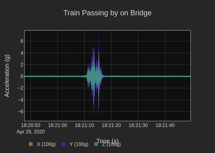
Now let's look at the real-world example of a train passing by on a bridge (discussed too in this blog). Figures 7 and 8 provide the time series overview.

Figure 7. Time-domain display showing three axes of vibration data from a bridge when a train is passing over
Figure 8. Expanded view of 100ms of time-domain vibration data
Figure 7 shows time-domain vibration data along the x-, y-, and z-axes. of a train passing over a bridge. The data consists of 10 seconds of 100,000 samples/s or a total of 1,000,000 samples, then Figure 8 shows a middle 100 ms of data or 10,000 samples. In the time domain, it is very difficult to see what frequency ranges are being excited!
Now let's determine the PSD of the three axes of acceleration by passing the time domain data to the PSD calculation function. In addition to the data, I will designate a 1 Hz bin width. Figure 9 presents the PSDs of the three orthogonal axes, both the still, and interactive image are provided!
Figure 9. X-axis, Y-axis, and Z-axis PSDs of the bridge vibration
If we examine the y-axis PSD. (Figure 9, remember zoom around!), we see a peak around 23 Hz which could be a fundamental mode of the bridge. Secondary peaks at other frequencies could be other resonances but they quickly become pretty broad, they aren't isolated to a single frequency. Using this PSD plot in a vibration simulation program can create a high level of complexity in the model.
Octave Spaced PSD
Our open-source software has an octave bin calculation program to widen the bin widths for the PSD, endaq.calc.psd.to_octave(). The program requires the starting frequency and the number of bins/octaves. Figure 10 shows the results of an octave PSD using a coarse 1 bin/octave.
Figure 10. The bridge PSD converted to 1/1 bins per octave spacing.
Determining what is the right number of bins per octave is up to the analyst. But this is one of the benefits of the PSD, it is a density so even as we change this bin width the value of the y-axis in the plots is held relatively constant. Let's compare a few different options in Figure 11. If I were the analyst I may want to use 6 (or maybe 3) but the 1/1 bins per octave gives a nice clean profile that is easy for a simulation software - but it's up to you!
Figure 11. PSDs with a different number of bins per octave.
Conclusion
Hopefully, now you can see how powerful the PSD information is for vibration analysis and understand how this calculation is done. Our open-source Python library simplifies the task of calculating the PSD and identifying frequencies where vibration magnitudes can be problematic. The PSD is an indispensable tool for vibration analysis. For further information on analyzing vibration data in the frequency domain, subscribe to our library of videos on the subject. Feel free to take advantage of our open-source Python library, it is free!
Please note: This post is the first of a four-post series. Be sure to subscribe to our blog if you'd like to receive the upcoming posts in your inbox.
- Calculate a PSD with Python
- Calculating a FFT from a PSD
- Comparing the FFT to PSD
- Time Varying Frequency Analysis