I was chatting with my colleague Steve Hanly about his recent post on the Fourier transform and power spectral density, and we thought it might help to go a bit more into the math and guts of the Fourier transform. As we know, the Fourier transform is a common and useful engineering tool for analyzing signals and vibrations, but sometimes it can produce some hard to interpret results.
My aim for this post is to start things off with a refresher on the basics of the math behind the Fourier transformation, and lay the foundation for future posts that will go into more detail on how the Fourier transform should be used and interpreted.
Complex Numbers: Magnitude, Angle, and Euler's Formula
A complex number has separate real and imaginary components, such as the number 2 + j3. The letter j here is the imaginary number, which is equal to the square root of -1. I will use j as the imaginary number, as is more common in engineering, instead of the letter i, which is used in math and physics.
Complex numbers have a magnitude:
![]()
And an angle:
![]()
A key property of complex numbers is called Euler’s formula, which states:
![]()
This exponential representation is very common with the Fourier transform. Note that an imaginary number of the format R + jI can be written as Aejξ where A is the magnitude and ξ is the angle.
The Continuous Time Fourier Transform
Continuous Fourier Equation
The Fourier transform is defined by the equation
![]()
And the inverse is
![]()
These equations allow us to see what frequencies exist in the signal x(t). A more technical phrasing of this is to say these equations allow us to translate a signal between the time domain to the frequency domain. Note that these equations use a ξ (the Greek letter Xi) to imply frequency instead of ω (Omega) which generally refers to angular frequency (ω = 2πξ). The Fourier transform of a time dependent signal produces a frequency dependent function.
A lot of engineers use omega because it is used in transfer functions, but here we are just looking at frequency. If we use the angular frequency instead of frequency, then we would have to apply a factor of 2π to either the transform or the inverse. The general rule is that the unit of the Fourier transform variable is the inverse of the original function’s variable.
Example Transformations
Let’s kick these equations around a bit. Let’s try the super simple function x(t) = 2. Plugging this equation into the Fourier transform, we get:
![]()
Integrals around infinity start to behave oddly, so this example will not be mathematically rigorous, but intuitively we can see that the integral of sin(ξt) and cos(ξt) as t goes from negative infinity to positive infinity should be 0, unless ξ = 0. At that point the equation simplified dramatically to:
![]()
We can write the equation for X(ξ) using the Dirac delta function, δ(x), which is defined as:
![]()
So, putting it all together, for x(t) = 2, X(ξ) = 2 δ(ξ). This means that the magnitude of X(ξ) is 0 everywhere except at ξ=0, where it is roughly 2∞. A more mathematically rigorous process rests on the transform of the unit step function, which rests on the transform of an exponential decay. The purpose here is just to show that the transform of a DC signal will exist only at 0 Hz.
Now let’s look at the Fourier transform of a sine wave of frequency 1kHz.
![]()
We can see that this is going to come to zero except for the case where ξ=±1000. At that point, using ξ=1000 for this example, the equation becomes:
We can apply the trigonometric identity of sin(kt)cos(kt) = sin(2kt)/2 and sin2(kt) = (1-cos(2kt))/2, and we get:
![]()
![]()
Similarly, at ξ=-1000, we will get:
![]()
Using the Dirac function, we see that the Fourier transform of a 1kHz sine wave is:
![]()
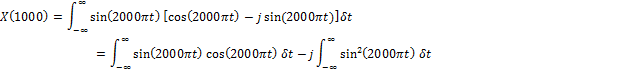
We can use the same methods to take the Fourier transform of cos(4000πt), and get:
![]()
A few things jump out here. The first is that the Dirac function has an offset, which means we get the same spike that we saw for x(t) = 2, but this time we have spikes at the signal frequency and the negative of the signal frequency. This makes more sense when you remember that sin(-θ) = -sin(θ), and cos(-θ) = cos(θ). The second piece that should jump out is that the Fourier transform of the sine function is completely imaginary, while the cosine function only has real parts. This means that the angle of the transform of the sine function, which is the arctan of real over imaginary, is 90° off from the transform of the cosine, just like the sine and cosine functions are 90° off from each other.
Convolution and Linearity
The Fourier transform is linear, meaning that the transform of Ax(t) + By(t) is AX(ξ) + BY(ξ), where A and B are constants, and X and Y are the transforms of x and y. This property may seem obvious, but it needs to be explicitly stated because it underpins many of the uses of the transform, which I’ll get to later. One property the Fourier transform does not have is that the transform of the product of functions is not the same as the product of the transforms. Or, stated more simply:
![]()
![]()
The Fourier transform of the product of two signals is the convolution of the two signals, which is noted by an asterix (*), and defined as:
![]()
This is a bit complicated, so let’s try this out. We’ll take the Fourier transform of cos(1000πt)cos(3000πt). We know the transform of a cosine, so we can use convolution to see that we should get:
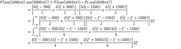
A long equation, but since δ(x) = 0 where x ≠0, we can see that there are only a few spots where we get non-zero answers. For example, in the first term we have:
![]()
For δ(ξ’-500) to be non-zero, we need to set ξ’=500. Then we have δ(ξ - ξ’ - 1500) = δ(ξ – 500 - 1500) = δ(ξ - 2000), so at frequency 2000 we have a value of δ(0)/2. We can continue this for all 4 terms and see that we get the same result at frequency 2000, 1000, -1000, and -2000. What happened here? We multiplied two frequencies together and the result is that we essentially re-centered the response for one at the frequency of the other. cos(1000πt) gives spikes at 500 and -500 Hz, cos(3000πt) works at 1500 and -1500 Hz, so we took the ±500 Hz spikes and re-centered them at 1500 and -1500 Hz. Similarly, if we take any waveform and multiply it by a sine or cosine, the transform of the resulting signal is the original re-centered at the frequencies of the sine wave. This is a very important feature that can easily get confusing, so I’ll cover it more in future posts.
The Discrete Time Fourier Transform
How to Use the Discrete Fourier Transform
The discrete Fourier transform (DFT) is the most direct way to apply the Fourier transform. To use it, you just sample some data points, apply the equation, and analyze the results. Sampling a signal takes it from the continuous time domain into discrete time. Here, I’ll use square brackets, [], instead of parentheses, (), to show discrete vs continuous time functions. The input to a discrete function must be a whole number. Sampling a signal x(t) at sample period Ts will turn it into x[n] such that:
x[n]=x(nTs)
So a sine wave of frequency fs = 1kHz sampled at Ts = 10uS will become:
x[n] = sin(2πfsnTs) = sin(0.02πn)
I’m using n instead of t to denote that we are just looking at a sequence of points; there is no inherent time signature here. A 100 Hz sine wave sampled at 1kHz looks exactly like a 10 Hz sine wave sampled at 100 Hz.
Discrete Fourier Equation
A common form of the DFT equation is
![]()
Here, N is the total number of points included in the equation, and m, the input to the transformed function, roughly correlates to the frequency in the same way that n correlates to time with the equation:
![]()
Let’s say we’re gathering 10 samples sampled at 100uS. For an input signal of x(t)=2, we will get x(0) = 2, x(1) = 2, x(2) = 2, etc. Plugging this into the DFT, we get:
![]()
![]()
|
n |
Real Results |
Imaginary Results |
|
0 |
1 |
- j0 |
|
1 |
+ 0.809017 |
- j0.587785 |
|
2 |
+ 0.309017 |
- j0.951057 |
|
3 |
- 0.30902 |
- j0.951057 |
|
4 |
- 0.80902 |
- j0.587785 |
|
5 |
- 1 |
- j0 |
|
6 |
- 0.80902 |
+ j0.58779 |
|
7 |
- 0.30902 |
+ j0.95106 |
|
8 |
+ 0.309017 |
+ j0.95106 |
|
9 |
+ 0.809017 |
+ j0.58779 |
X[1] = 0 - j0
As we expect, the sum of a sine and cosine over the whole period equals 0. We can assume that all other values of m will similarly be 0, so, similar to the time domain example, we have:
![]()
To get the actual signal magnitude we need to divide by N.
Let’s make things more complicated and take the DFT of the following signal, using 10 points sampled at 100 uS:
![]()
![]()
Running this through the DFT equation will get us the following values:
|
Sample |
Real Results |
Imaginary Results |
|
X[0] |
0 |
- j0 |
|
X[1] |
0 |
- j5 |
|
X[2] |
0 |
- j0 |
|
X[3] |
0 |
- j0 |
|
X[4] |
3.535534 |
- j3.535534 |
|
X[5] |
0 |
- j0 |
|
X[6] |
3.535534 |
+ j3.535534 |
|
X[7] |
0 |
- j0 |
|
X[8] |
0 |
- j0 |
|
X[9] |
0 |
+ j5 |
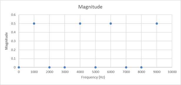
As we expect, the two sine waves show up clearly, although their magnitude needs to be normalized by the number of samples taken. We can find the frequency of the signals using the mfs/N equation, using fs = 1/100 uS = 10kHz, and N = 10, so m=1 corresponds to 1kHz, m=4 is 4kHz, m=6 is 6kHz, and m=9 is 9kHz. These high frequency results are really ghost images, similar to how we saw sine and cosine waves showing up at positive and negative frequencies. This also serves to illustrate the problem of aliasing, where higher signals above fs/2 appear as lower frequency signals. Just as out 1 kHz signal shows up at 9kHz, a 9kHz signal can show up at 1kHz. The second half of a DFT is generally left off because it tends to not contain any new information. This post will leave it in because it does help to illustrate some points.
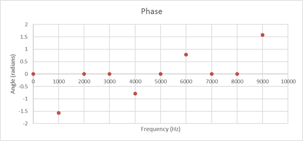
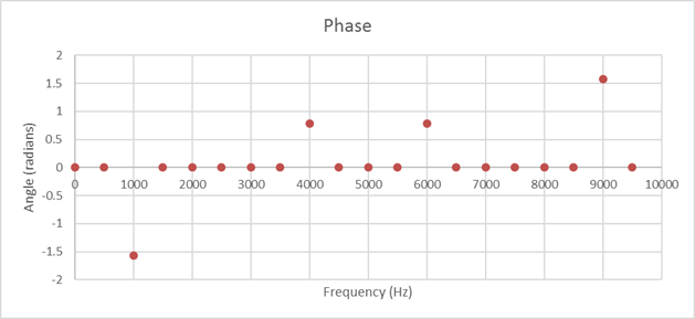
The angle of the 1kHz component is 90°, while the angle for the 4kHz component is 45°, or π/4 radians, corresponding to the phase shift of the actual signal.
Next, let’s try taking more samples with the same signals. If we keep the signal frequencies and sample rate the same, but increase the number of samples from 10 to 20, we get parameters of:
|
Sample |
Re |
Im |
Freq |
Sample |
Re |
Im |
Freq |
|
X[0] |
0 |
j0 |
0 Hz |
X[10] |
0 |
j0 |
5.0 kHz |
|
X[1] |
0 |
j0 |
0.5 kHz |
X[11] |
0 |
j0 |
5.5 kHz |
|
X[2] |
0 |
-j10 |
1.0 kHz |
X[12] |
7.07 |
j7.07 |
6.0 kHz |
|
X[3] |
0 |
j0 |
1.5 kHz |
X[13] |
0 |
j0 |
6.5 kHz |
|
X[4] |
0 |
j0 |
2.0 kHz |
X[14] |
0 |
j0 |
7.0 kHz |
|
X[5] |
0 |
j0 |
2.5 kHz |
X[15] |
0 |
j0 |
7.5 kHz |
|
X[6] |
0 |
j0 |
3.0 kHz |
X[16] |
0 |
j0 |
8.0 kHz |
|
X[7] |
0 |
j0 |
3.5 kHz |
X[17] |
0 |
j0 |
8.5 kHz |
|
X[8] |
7.07 |
j7.07 |
4.0 kHz |
X[18] |
0 |
j10 |
9.0 kHz |
|
X[9] |
0 |
j0 |
4.5 kHz |
X[19] |
0 |
j0 |
9.5 kHz |

So far, so good! The discrete Fourier transform has a few complexities, but it should all look familiar based on our understanding of the continuous time Fourier transform. In my next post, I’ll get into leakage, which is what happens when the signal, number of samples, and sample frequency all start to drift apart, and how we can solve that.
Check out my latest blog: Frequency Leakage in Fourier Transforms.