Filter Selection for Shock and Vibration Applications

Filtering is used to remove unwanted frequency content and should be an important part of your evaluation of different DAQ systems.  But which filter type is best for your application?

In this blog I'll highlight why filtering is important; but I'll also compare four types that are commonly used in shock and vibration testing:

• Butterworth
• Bessel
• Chebyshev
• Elliptical

At the end of the post I'll provide some resources for additional information.  All the MATLAB code used to generate these plots is also available and embedded in the blog.

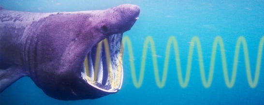
Anti-Aliasing

High-pass filters remove lower frequency vibration and is inherent to all piezoelectric accelerometers (resistor and capacitor in series) which gives these accelerometers the AC response (for more information on acceleroemter types check out our blog on accelerometer selection). This is useful for filtering out DC bias and the drift that can often occur due to temperature change.

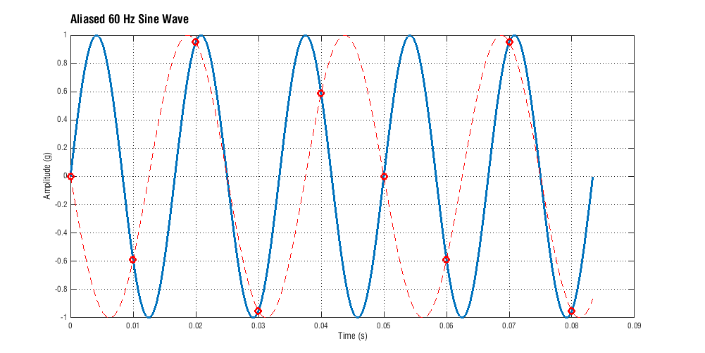
Low-pass filters are more important however to prevent aliasing which can’t be filtered out in software. Aliasing causes a signal to become indistinguishable or to look like a completely different signal as shown in Figure 1. It’s important to realize that an analog lowpass filter is needed to prevent aliasing. Once a signal is aliased, it can’t be filtered out digitally in software.

Filter Types

Now the question remains as to what type of filter should you use? An ideal filter would uniformly pass all frequencies below a specified limit and eliminate all above that limit. This ideal filter would have a perfectly linear phase response to the same upper frequency limit. But ideal filters don’t exist; there is some compromise that needs to be made on a filter’s amplitude and phase response. There are four main different types of filters:

Butterworth

A Butterworth filter is known for its maximally flat amplitude response and a reasonably linear phase response. The Butterworth filter is the most popular for vibration testing.

Bessel

The Bessel filter has nearly perfect phase linearity so it is best suited for transient events like shock testing. It has a fairly good amplitude response but its amplitude roll-off is slower than the Butterworth or Chebyshev filter.

Chebyshev

The Chebyshev has a faster roll-off in the amplitude response which is achieved by introducing a ripple before the roll-off. They have a relatively nonlinear phase response.

Elliptic

The Elliptical filter has the steepest roll-off in the amplitude response but it has a ripple in both the pass band and stop band. In addition, its phase response is highly nonlinear. This is only used for applications where phase shift or ringing is not of a concern; it should generally be avoided to the common test engineer because of its tendency to distort complex time signals.

Filter Comparison

In Figure 2 the performance of these filters are compared for a 1,000 Hz cut off frequency and 5^th order filters. 

Figure 3 takes a closer look at the filter performance in the passband (0 to 1,000 Hz). The Chebyshev and Elliptical filters offer that sharper amplitude roll off but at the expense of large ripples in the passband and nonlinearity. Butterworth filters offer the best of both worlds with a relatively sharp amplitude roll off. Bessel has the best phase response and a reasonably good amplitude response but note how early it begins filtering!

Notice how all the filter types begin attenuating the signal before the cut-off frequency.  This is because the cut-off frequency of a filter specifies when the attenuation has reached -3dB which is nearly -30%!

The Code

The plots were generated in MATLAB using the Signal Processing Toolbox and the analog filter functions.  The code used is included below.

close all
clear all

%Define Variables
    n = 5; %fifth order
    f = 1000; %filter frequency
    np = 2^12; %number of points
    fig = figure('Position', [100, 100, 600, 600]);

%Butterworth
    [b,a] = butter(n,2*pi*f,'s');
    [h,w] = freqs(b,a,np);
    phasedeg = unwrap(angle(h))*180/pi;
    w = w/(2*pi);
    subplot(2,1,1)
        hold all
        grid on
        plot(w,abs(h),'Linewidth',2)
        set(gca,'YScale','log');
        xlabel('Frequency (Hz)')
        ylabel('Attenuation')
        title('Amplitude Response of 1,000 Hz Filter')
    subplot(2,1,2)
        hold all
        grid on
        plot(w,phasedeg,'Linewidth',2)    
        %(gca,'XScale','log');
        xlabel('Frequency (Hz)')
        ylabel('Phase (degrees)')      
        title('Phase Response of 1,000 Hz Filter')
        
%Bessel
    [b2,a2] = besself(n,2*pi*f*1.62);
    [h2,w2] = freqs(b2,a2,np);
    phasedeg2 = unwrap(angle(h2))*180/pi;
    w2 = w2/(2*pi);
    subplot(2,1,1)
        plot(w2,abs(h2),'Linewidth',2)
    subplot(2,1,2)
        plot(w2,phasedeg2,'Linewidth',2)    

%Cheby1
    [b3,a3] = cheby1(n,3,2*pi*f,'s');
    [h3,w3] = freqs(b3,a3,np);
    phasedeg3 = unwrap(angle(h3)*180/pi);
    w3 = w3/(2*pi);
    subplot(2,1,1)
        plot(w3,abs(h3))
    subplot(2,1,2)
        plot(w3,phasedeg3)           
         
%Cheby2
    [b5,a5] = cheby2(n,30,2*pi*f,'s');
    [h5,w5] = freqs(b5,a5,np);
    phasedeg5 = unwrap(angle(h5)*180/pi);
    w5 = w5/(2*pi);
    subplot(2,1,1)
        plot(w5,abs(h5))
    subplot(2,1,2)
        plot(w5,phasedeg5)            

%Elliptical    
    [b4,a4] = ellip(n,3,30,2*pi*f,'s');
    [h4,w4] = freqs(b4,a4,np); 
    phasedeg4 = unwrap(angle(h4))*180/pi;
    w4 = w4/(2*pi);
    phasedeg4(w4>=1065) = phasedeg4(w4>=1065) -180;
    phasedeg4(w4>=1333) = phasedeg4(w4>=1333) -180;
    
%Finish plotting and format
    subplot(2,1,1)
        plot(w4,abs(h4))
        axis([0 5*f .001 1])
        set(gca, 'YTickLabel', {'0.001','0.01', '0.1', '1'})
        legend('butter','bessel','cheby1','cheby2','ellip','Location','northeast')
        ax1 = gca;
        ax1_pos = ax1.Position; % position of first axes
    ax2 = axes('Position',ax1_pos,...
        'XAxisLocation','top',...
        'YAxisLocation','right',...
        'Color','none');
        grid(ax2,'off')
        set(ax2,'xlim',[0 2*f])
        set(ax2,'xticklabel',{'','','','',''})
        set(ax2,'ylim',[0.001 1])
        set(ax2,'yscale','log')
        set(ax2,'ytick',[0.001 0.01 .1 1])
        set(ax2,'yticklabel',{'-60 dB','-40 dB','-20 dB','  0 dB'})
    subplot(2,1,2)
        plot(w4,phasedeg4)  
        xlim([0 5*f])
        legend('butter','bessel','cheby1','cheby2','ellip','Location','northeast')

Conclusion

Which filter you choose will depend on your application; but in general, the Butterworth filter is best for vibration and the Bessel is best for shock testing. And above all, you should avoid a system that does not offer some low pass filtering to prevent aliasing.

For a deeper dive into filters for vibration and shock testing, check out Strether's post on different anti-alias filters.

If you'd like to learn a little more about various aspects in shock and vibration testing and analysis, download our free Shock & Vibration Testing Overview eBook.  In there are some examples, background, and a ton of links to where you can learn more.  And as always, don't hesitate to reach out to us if you have any questions!