Comparing the Fourier Transform, the Power Spectral Density, and the Aggregate FFT for Vibration Analysis

The Fourier transform, a power spectral density (PSD), and the aggregate fast Fourier transform (FFT) are three methods that you can use to analyze the frequency components of a waveform, such as a vibration waveform. Each method has its advantages and disadvantages for analyzing different types of waveforms. I will compare the three analysis methods using both some simulated data and some actual vibration data using the enDAQ open-source library routines.  

In this post, I will present:

1. Content of the simulated data
2. Analyzing the data using the FFT method
3. Analyzing the data using the PSD method
4. Analyzing the data using the Aggregate FFT method
5. Using the simulated data to compare the three methods
6. Using the three techniques on real-world data
7. Summary and suggested protocol for analysis

Video Presentation

Content of the simulated data  

The simulated acceleration data consists of a combination of three signals. The first signal is white noise, a fairly constant amplitude, from 10 Hz to 50 Hz. The second and third signals are a 30 Hz sine tone and an 80.25 sine tone. The two sine tones each have a magnitude of 1 g. I have combined 10 seconds of each waveform. Figure 1 shows the resulting time domain plot of the combined signals, and Figure 2 shows the time domain plot of the random noise which is not visible in Figure 1. Figure 3 shows the time domain data of the sine tones. While the plots give an indication of the amplitude of the data, they do not give any information on the frequency content of the data. 

Figure 1. Analog time domain plot of the random noise (yellow curve, mostly hidden), the 30 Hz and 80.25 Hz sine tones (blue curve), and the combination of the three waveforms (green) 

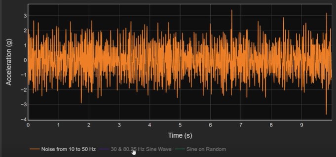
Figure 2. Time domain plot of the 10 Hz to 50 Hz random noise  

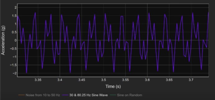
Figure 3. Time domain plot of the 30 Hz and 80.25 Hz sine tones

Analyzing the data using the FFT method

The first method I will use to analyze the frequency content of the data is the computation of the Fourier transform on the data using a FFT methodology. I will display the real component of the Fourier transform. Figure 4 shows the results of the Fourier analysis. I am showing multiple analyses over six time intervals, and the plots are overlaid on each other. If I isolate on the 10 s time interval, FFT analysis (Figure 5), the plots contain the near-constant amplitude of the 10-to-50 Hz noise and two spikes representing the 30 Hz and 80.25 sine tones. The middle plot displays the 30 Hz tone with a magnitude of 1 g which is what you would expect to see. The 80.25 Hz tone only has a magnitude of 0.6 g. That is a function of the width of the frequency divisions or bins that I have chosen for the Fourier transform computation. The 80.25 sine tone does not fit entirely in one frequency bin. The amplitude of the tone leaks into adjacent bins. While the 30 Hz tone fits neatly into one bin and is displayed as a narrow triangle with an amplitude of 1 g. the 80.25 tone is a wider signal with signal content in more than one frequency bin. 

Now if we look at the partial time interval, the 0-to-1 s analysis (Figure 6), we get an entirely different display. This illustrates that the FFT data is a function of the time interval, which determines the frequency bin width, and how well the bins align with the frequency of signal spikes.  

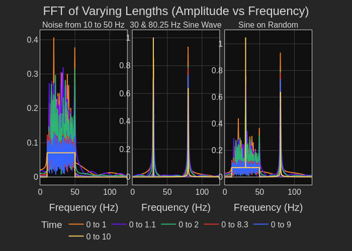
Figure 4. FFT analysis of the 10-to-50 Hz noise, the 30 Hz and 80.25 Hz sine tones, and the combination of the three signals 

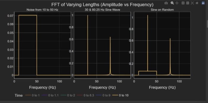
Figure 5. FFT computation using the full 10 s of data 

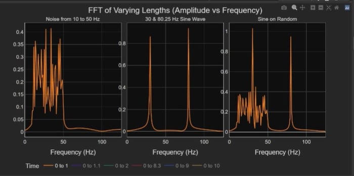
Figure 6. FFT analysis on 1 sec of data. Note the amplitude of the sign tones are different in this plot compared with the 10 s time interval in Figure 5. 

Analyzing the data using the PSD method

Now let me compute the power spectral density of the time domain data. Figure 7 displays the plot of the PSD analysis of the data over the same six time intervals used to compute the FFT. Again, the noise and the sine tone PSD’s are displayed separately. The right-side plot of Figure 7 includes the analysis of the combination of the three signals. Each row shows the results of the analysis using increasing bin widths. As the bin width increases, the amplitude of the noise data remains constant; but the sine tone amplitudes vary. Now let me plot the 0 to 10 s segment of the data on top of the 0 to 2 s data (Figure 8). You can see that there is no change in the data. The peak amplitudes are independent of the time range. In fact, the amplitude of the random content is independent not just of the time range but also the selected frequency bin width. The reason is this is power density function, essentially the square of the Fourier transform; and, it spans all the frequency content. Thus by widening the bin width, you are filtering the data and smoothing the amplitudes; however, the average amplitude remains the same value. While the random noise amplitude is independent of bin width, the same is not true of the sine tones. The other negative with the PSD is that the amplitude of the results is no longer the units of the original analog data, in this case units of acceleration, g.  

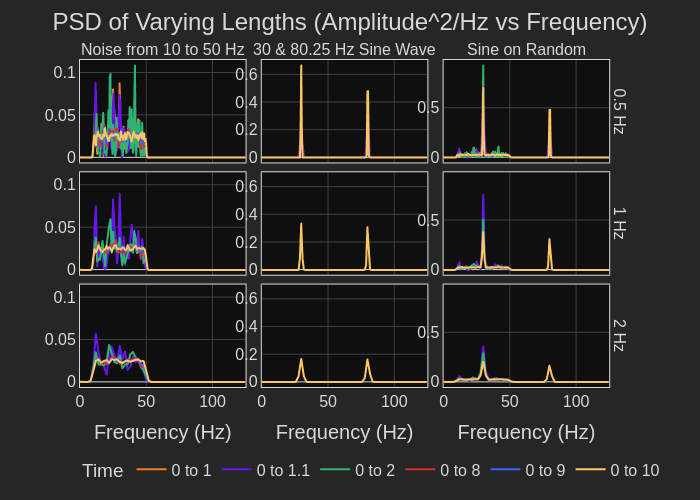
Figure 7. PSD data analyzed over six time intervals and three different bin widths 

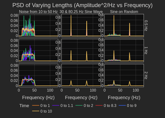
Figure 8. PSD over 2 s (green plot) and 10 s (yellow plot) 

Analyzing the data using the Aggregate FFT method 

Let’s take a look at the results from an aggregate FFT computation. This method segments the data file into overlapping time intervals. The FFTs of the segments are computed and then averaged. See Figure 9. One benefit, similar to the PSD, is that the results are independent of the time interval selected. See Fig 10. The peaks at 30 Hz and 80.25 Hz are now what we would expect. The peak at 30 Hz has an amplitude of 1 g, the true amplitude of the 30 Hz sine tone. The 80.25 Hz sine tone shows up a little less than its amplitude of 1 g, due to the frequency of the sine tone not fitting perfectly in to 1 bin as I indicated when discussing the Fourier transform computation. While the aggregate FFT presents the sine tones more accurately, the amplitude of the noise spectrum changes as the bin width changes. As the frequency bin width widens to include more frequency content in each bin, the amplitude of the noise spectrum increases. Thus the aggregate FFT accurately captures individual sine tone magnitudes, but the noise spectrum amplitude is a function of the bin width selected.  

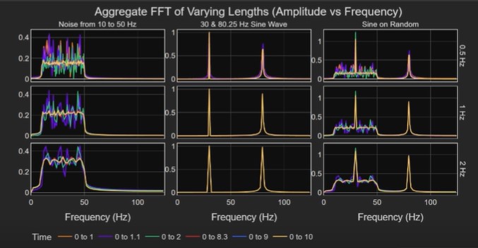
Figure 9. Overlays of Aggregate FFT data over six time intervals and three frequency bin widths 

Figure 10. The Aggregate FFT over the 2 s interval (green plot) and the 10 s interval (yellow plot) as a function of the individual signals and the three bin widths 

Using the simulated data to Compare the three methods  

Figure 11 compares the three analysis methods over different time ranges and bin widths. Let’s look at the plot of the aggregate FFT data at the 0-to-10 s time interval and with a 2 Hz bin width (Figure 12). The plot shows the amplitude of the 80.25 Hz sine tone as about 1 g. The 2 Hz bin width includes all the frequency content of the 80.25 Hz sine tone. The Fourier transform plot, whose bin width is a function of the time length of the data analyzed, shows a much lower amplitude for the 80.25 sine tone. The Fourier transform, with the 10 s time interval, used 0.5 Hz bin widths. So, half of the 80.25 Hz sine tone is in each of the 80.0 Hz and 80.5 bins.  

For capturing spikes of narrow frequency content, the Aggregate FFT analysis is superior to the Fourier transform analysis whose bin width is determined by the data time interval. The Aggregate FFT allows independent selection of bin width. The PSD normalizes the frequency bin width so the results for random noise data are independent of time interval and bin width. However, in all three computation methods, bin width impacts the amplitude of the sine tones.  

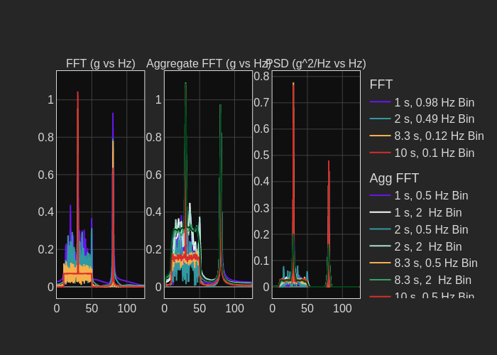
Figure 11. Comparison of the three analysis methods over various combinations of time interval and frequency bin width. The various curves are overlaid on each other. 

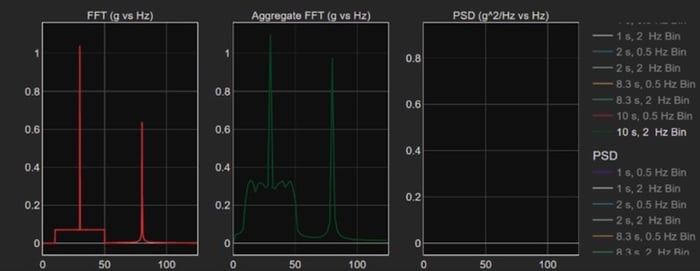
Figure 12. The Aggregate FFT plot (green data) with a 2 s time interval and a 2 Hz bin width and a 10 s interval FFT plot (red data). Note the difference in the amplitude of the 80.25 Hz sine tone in the FFT plot vs the Aggregate FFT plot.  

Using the three techniques on real-world data 

Now I am going to analyze some real-world data. This data file is an hour of x-, y-, and z-axis components of vibration data on a prototype device subjected to a Mil Standard 810 vibration profile. I added three sine tones to the data file. The three sine tones are at 30 Hz, 80.25 Hz, and 300.5 Hz. One hour of data is a huge amount of data so I will extract 1 s of the analog data (see Figure 13). The plots show the vibration data, which is primarily x-axis vibrations, and the sine tones, the red line, added to the x-axis data. The analog, time domain data, as expected, does not yield any useful information. The sine tones are not visible in the plot. 

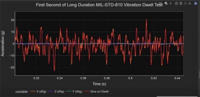
Figure 13. One second of analog data of a Mil Standard 810 vibration test along the x-axis (yellow plot). Three sine tones at 30 Hz, 80.25 Hz, and 300.5 Hz are combined with the Mil Standard data (red plot). 

If I calculate the PSD and plot it, you can see the Mil Standard 810 profile by itself (Figure 14). Then I have added the sine tones with the Mil Standard 810 profile in Figure15. However, the sine tones are not at the values that I expect.   

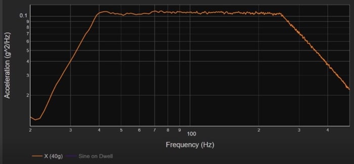
Figure 14. PSD of Mil Standard 810 vibration data 

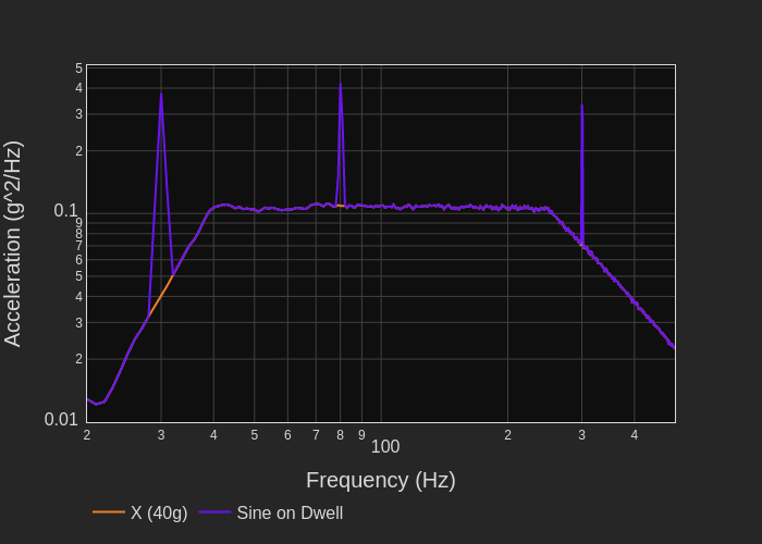
Figure 15. PSD of both the Mil Standard 810 profile and the three sine tones 

Now I will compare the results using the three techniques at combinations of different time intervals and different bin widths. I will analyze the x-axis data. Figure 16 shows the results of the three techniques. Waveforms at different time interval and bin width combinations for each technique are overlaid on each other.  

Let’s focus on the Fourier transform analysis method first. The purple plot of Figure 17b shows 1 s of data with a 1 Hz bin width. With a FFT computation, you cannot independently specify the bin width. The time length of the input data determines the effective bin width. The blue plot in Figure 17b shows 10 s of data with a resulting 0.1 Hz bin width. The 1 s and the 10 s curves are quite a bit different, but neither uncovers significant information. Now at 600 s and 3000 s, you can make out the random data and the sine tones (Figure 17c). However, the amplitudes are significantly different. The Fourier transform output does not accurately quantify the magnitudes and the plots can vary substantially as a function of bin width. 

Figure 16. Analysis of the vibration data and the sine tones using the three techniques. Results at various time intervals and bin widths are overlaid on each other.  

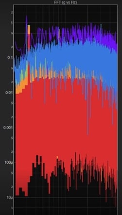
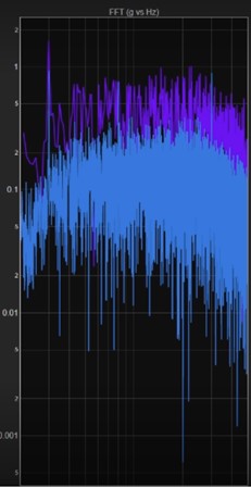
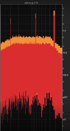
Figure 17. FFT analysis of the Mil Standard 810 data and the three sine tones 

Let’s take a look at the aggregate FFT analysis. Figure 18a shows the 10 s time interval, 1 Hz bin width result (blue curve) and the 10 s, 8 Hz bin width result (white curve). If I use a longer time interval of 60 s with a 1 Hz bin width, you can clearly see the 30 Hz, the 80.25 Hz, and the 300.5 Hz sine tones (Figure 18b). The amplitude of the 300.5 sine tone is much smaller than the 30 Hz and 80.25 Hz sine tones because the 300.25 Hz sine tone bleeds into two bins. I can clean the results up more by including more data with a longer time interval. In Figure 18c, I am showing the plots of 3000 s with an 8 Hz bin width (green curve) and 3000 s with a 1 Hz bin width (red curve). The 8 Hz bin width data averages the frequency content so that the sine tones are no longer clearly defined. I am using the large, 8 Hz bin width to illustrate how a change in bin width affects both the amplitude of the sine tones and the shape of the random data. The limitation of the Aggregate FFT analysis method is that the results are not normalized to the bin width. The advantage of the Aggregate FFT technique is that you can get a very clean plot. With reasonable bin widths, this method provides accurate magnitudes for the sine tones, but the method does not provide the best analysis for the random vibration data.  

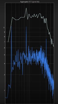
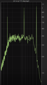
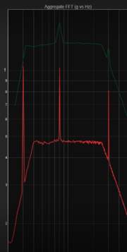
Figure 18. Aggregate FFT analysis of the Mil Standard 810 data and the three sine tones 

Let’s view the results of the third technique, the PSD analysis. Figure 19 repeats the PSD plots of the overlaid results for the various combinations of time intervals and bin widths. The shorter time intervals show plots with large amplitude variations in the Mil Standard, x-axis vibration data. With 60 s of data, the amplitude variations are smaller as shown in Figure 20. The green plot is the result with a 1 Hz bin width, while the blue plot shows how the results change with the wide 8 Hz bandwidth. Too wide a bin highly distorts the results, even with the PSD, as the blue plot demonstrates. The results improve with a 600 s time interval (Figure 21). As shown in Figure 22, the plot of 3000 s overlaid on the 600 s curve does not show any further improvement in reducing amplitude variation in the Mil Standard vibration data.  

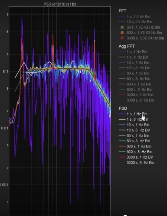
Figure 19. Ten PSD plots at increasing time intervals at 1 Hz and 8 Hz bin widths 

The limitation of the PSD analysis technique is that, due to the fact that it is a density computation, the technique can mask narrow frequency content signals if the selected bin width is too wide. Fortunately, most real-world, narrow frequency spikes will shift small amounts with time, temperature, drive frequency, and other factors. The spike will spread over a range of frequencies and the PSD analysis will identify the spike over a wider range of bin widths.

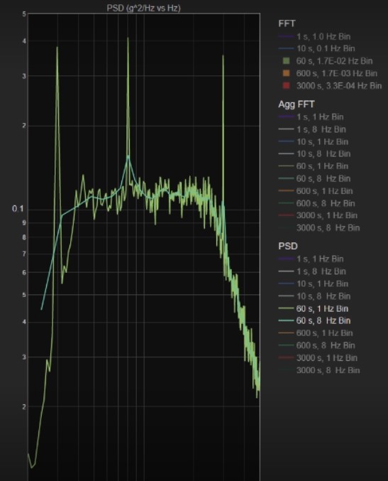
Figure 20. PSD analysis of 60 s of data at 1 Hz bin width (green plot) and 8 Hz bin width (blue plot) 

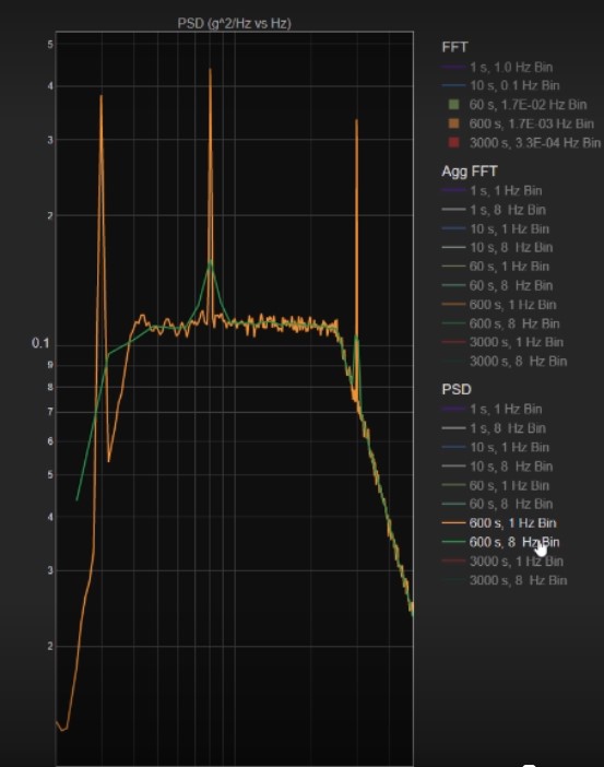
Figure 21. PSD plot of 600 s of data. The orange plot is the result using a 1 Hz bin width. The green plot is the result using an 8 Hz bin width. 

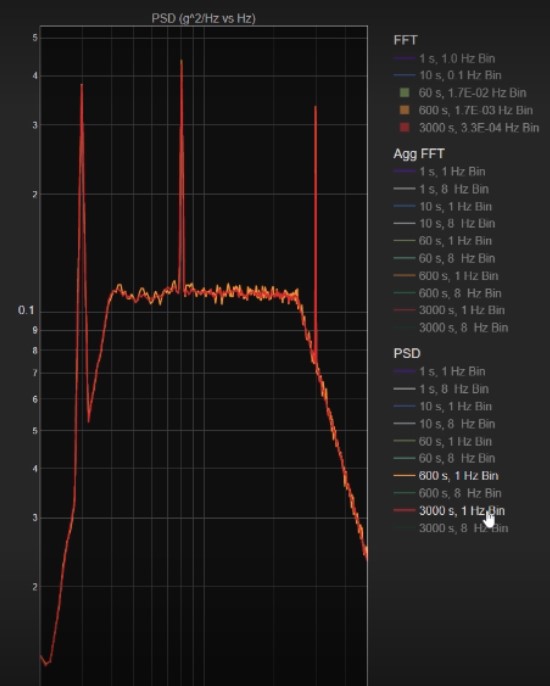
Figure 22. The 600 s data (orange plot) overlaid with the 3000 s data (red plot) 

Summary and suggested protocol for analysis 

Table 1 lists the three analysis techniques and summarizes the advantages and disadvantages of each technique. 

So which technique should you use? 

I suggest you use both the PSD and the Aggregate FFT.  The two methods complement each other. I recommend performing a PSD on your data first. It gives you the best results for random content, vibration analysis. However, if you notice a lot of narrow frequency spikes in your data, then also perform an Aggregate FFT analysis. Use a narrow bin width. See if you can identify sine tone peaks. The Aggregate FFT can tell you the amplitude of the sine tone peaks and their frequencies.  

Remember enDAQ’s analysis routines are open-source and available to you at {URL}. For more information on vibration analysis, subscribe to our video channel at {URL} and see more blogs at https://blog.endaq.com/.